PID Autotuning for UAV Quadcopter

UAV Package Delivery Model

In this example, a multirotor is modeled in Simulink® using UAV Toolbox components. This model is based on the UAV Toolbox uavPackageDelivery model. For more information, see UAV Package Delivery.

To get started, set up and open the Simulink Project.

prj = openProject('scdUAVPIDAutotuning');

Model Architecture and Conventions

The top model consists of the following subsystems and model references:

The model's design data is contained in a Simulink™ data dictionary in the data folder (uavPackageDeliveryDataDict.sldd). Additionally, the model uses variant subsystems to manage different configurations of the model. Variables placed in the base workspace configure these variants without the need to modify the data dictionary. For more details on variant subsystems, see What Are Variants? (Simulink).

PID Controller Autotuning

This example uses the Closed-Loop PID Autotuner (Simulink Control Design) block from Simulink Control Design™ software to tune eight controllers used in the attitude and position control of a multirotor. You can use many ways to tune controllers, including manual tuning and empirical calculations. By using the Closed-Loop PID Autotuner, you can set up the control system ahead of time and then perform tuning of all eight loops with a one-click process. This makes the entire tuning process repeatable and easily adjustable for future tuning. In this example, you use a six degree-of-freedom model of a multirotor in Simulink. However, you can also use the Closed-Loop PID Autotuner on hardware to perform the same process using a real multirotor. Most other tuning techniques are difficult to implement on actual multirotors, can take a long time, and are not easily repeatable.

By using the Closed-Loop PID Autotuner for tuning the controllers in this example you do not need to have advanced knowledge of control tuning techniques.

Modify UAV Package Delivery Model for PID Autotuning

To facilitate PID autotuning, the original UAV package delivery model is modified with these changes:

These changes allow for the multirotor to take off and remain at a fixed altitude while autotuning takes place and to update the gains of the PID Controllers, all in a single simulation.

Following Example Steps

Use the Project Shortcuts to step through the example. Each shortcut sets up the required variables for the project.

Getting Started

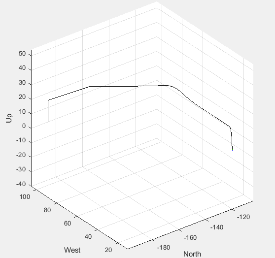
Click the Getting Started project shortcut, which sets up the model for a four-waypoint mission using a high-fidelity multirotor plant model. Run the uavPIDAutotuning model, which shows the multirotor takeoff, fly, and land in a 3-D plot.

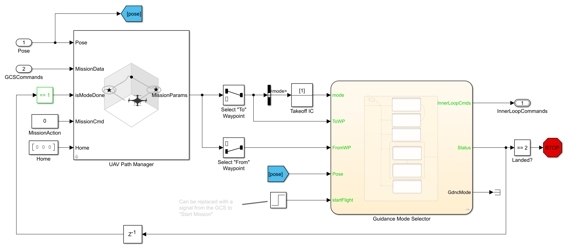
The model uses UAV Path Manager block to determine which is the active waypoint throughout the flight. The active waypoint is passed into the Guidance Mode Selector Stateflow® chart to generate the necessary inner loop control commands.

Use the Simulation Data Inspector to visualize the UAVState output of the multirotor model.

You can see that the multirotor takes almost 150 seconds to complete the four waypoint path with the baseline set of gains. In order to improve this performance, retune the PID Controllers used in the multirotor.

Run Autotuning Mission

Once you are able to fly a basic mission, you are ready to autotune the attitude and position control loops to improve the performance of the multirotor. The control system for this example contains eight PID Controllers. The system has four cascading control loops. Each loop contains two controllers, one for each axis. This diagram shows how the eight controllers are set up with the Closed-Loop PID Autotuner blocks in order to perform autotuning.

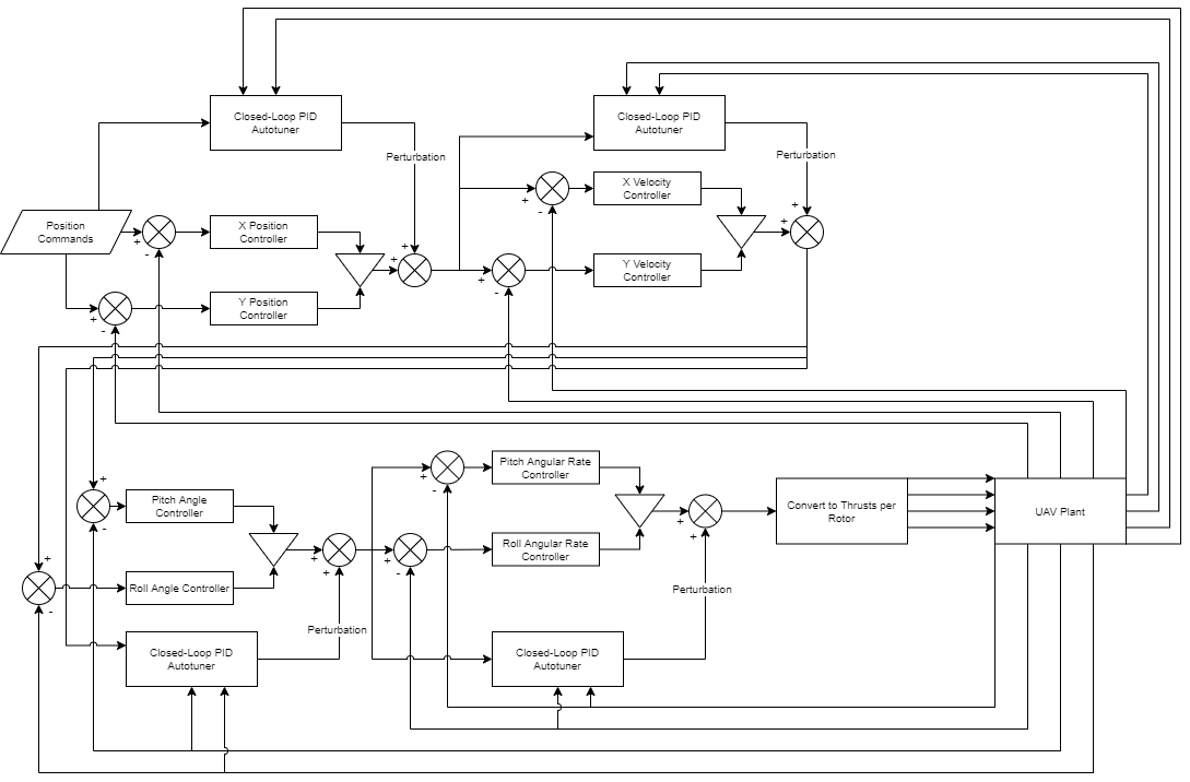
The Closed-Loop PID Autotuner blocks inject perturbation signals to the output of each of the eight existing PID Controllers. The autotuners then use the feedback signals and the output of the PID Controllers in order to perform the autotuning process. With the exception of the innermost control loops, pitch and roll rate, the two axes being controlled are decoupled from each other. For example, the x velocity and the y velocity loops are decoupled from each other. This allows you to tune these two loops simultaneously which reduces the overall time to perform autotuning. For the pitch rate and roll rate loops, tune the control loops sequentially because they are coupled. This results in the following sequence for tuning the PID Controllers:

Click the Autotune PID Controllers project shortcut, which sets up the model to hover at a low altitude and automatically tune the four PID Controllers, then runs the same four-waypoint mission from first step.

The Closed-Loop PID Autotuner blocks for each control loop are set up with different performance criteria depending on the control loop. For cascaded control, such as that used in this example, the inner loop should have a higher bandwidth than the outer loop to avoid instabilities. For this example, that means the pitch and roll rate control loops have the highest bandwidth while the x and y position control loops have the slowest bandwidths.

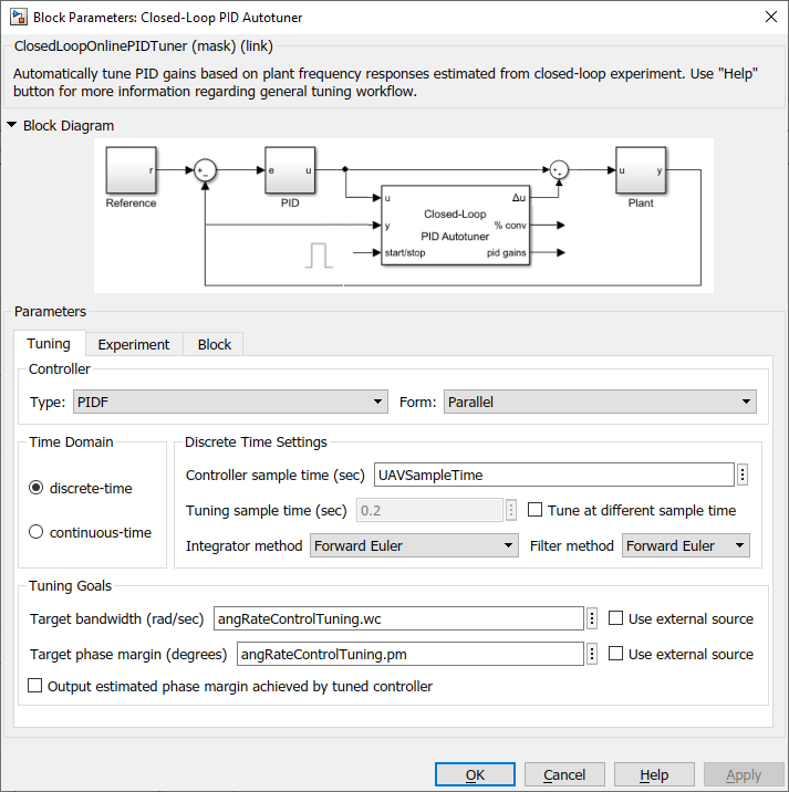
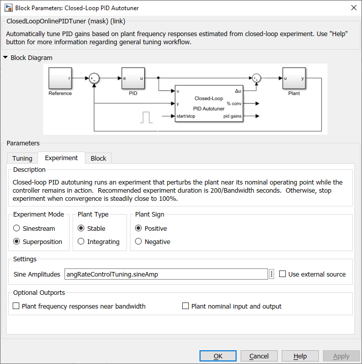
The settings used for the pitch and roll rate loops are:

The settings used for the pitch and roll loops are:

The settings used for the x and y velocity loops are:

The settings used for the x and y position loops are:

To maximize performance, the bandwidth for the pitch and roll rate loops is set to 50 rad/sec. The sampling time ${\mathit{T}}_{\mathit{s}}$ of the UAV control system is 0.005 seconds and the Closed-Loop PID Autotuner requires that the bandwidth $\omega$ must satisfy $\omega {\mathit{T}}_{\mathit{s}}\le 0.3$, which means that bandwidth must be 60 rad/sec or less. Choose the bandwidth such that it is less than the required 60 rad/sec. The other bandwidths are set to be as large as possible while not causing stability issues with inner loops.

The phase margin for each loop is set to 60 degrees as this value is typically a good compromise between performance and damping. This margin is the default setting for the Closed-Loop PID Autotuner block.

The perturbation amplitudes are set such that they are less than 5% of the maximum expected output of the individual controllers. If the value for the perturbations is too high, it can cause the multirotor to become unstable during tuning. If the value for the perturbations is too low, the autotuner might not get an accurate estimate of the plant and the calculated gains might not meet the desired bandwidth or phase margin.

The settings for the individual loops are contained in the data dictionary, uavPackageDeliveryDataDict.sldd. The following images show a sample of how to enter these settings in the Closed-Loop PID Autotuner blocks used to tune the pitch angular rate.

Run the uavPIDAutotuning model, which shows the multirotor takeoff, hover, autotune the PID Controllers, fly, and land in a 3-D plot.

Use the Simulation Data Inspector to visualize the UAVState output of the multirotor model.

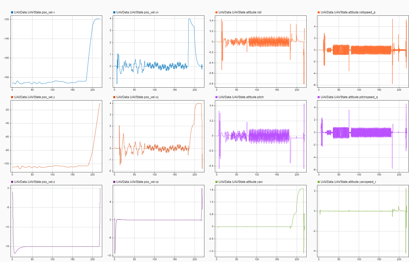
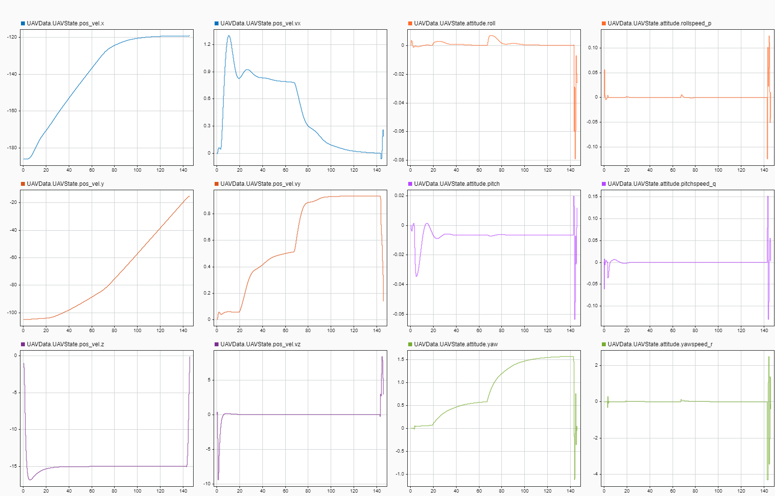
As you can see, the multirotor hovers for a period of time in order to perform autotuning. After the autotuning process is complete, around 185 seconds into the simulation, the multirotor follows the same four-waypoint path as in project first step, but the quadcopter is able to complete the path in a much shorter time due to the tuned gains increasing performance.

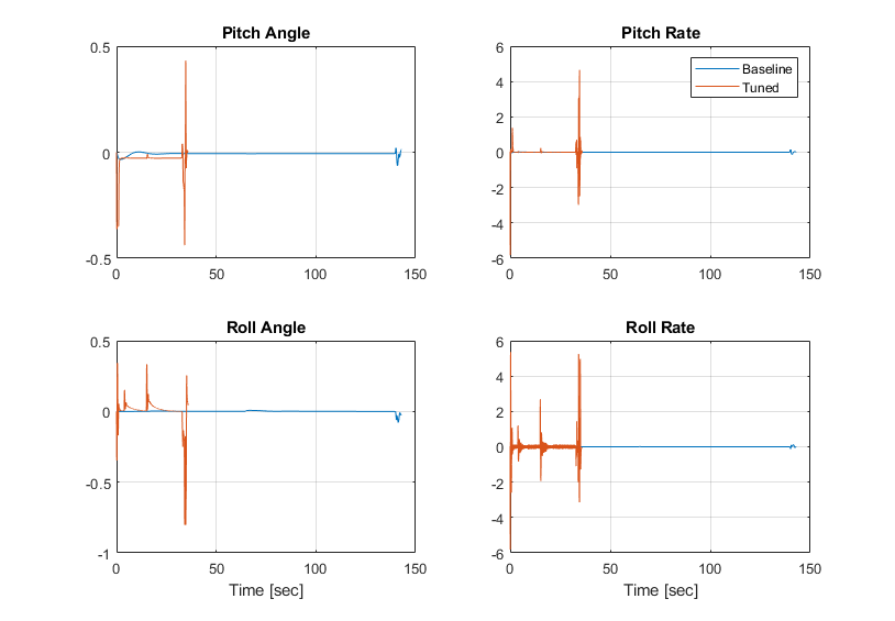
These plots show the position and attitude responses for the multirotor over the path. The blue line shows the multirotor performance with the baseline set of gains while the red line shows the multirotor performance with the tuned gains. With the tuned set of gains, the multirotor is able to complete the path in about 45 seconds. Meanwhile, with the baseline set of gains, the multirotor takes almost 150 seconds.

During the autotuning process the gains are updated for the eight controllers:

Autotuning Altitude and Heading/Yaw Control Loops

In this example you learned how to automatically tune the P, I, D and N gains for four separate paired control loops used for the attitude and position control. However, this example model contains two more control loops, one for altitude and one for the heading or yaw angle. Using the same methodology for autotuning presented in this example, you can add the Closed-Loop PID Autotuner to one or both of these other control loops and perform the autotuning process.

In order to tune the controllers for either of these loops, ensure that the tuning happens only when the tuning is not running for the other controllers. You can either disable tuning of the other controllers or you can tune these controllers after tuning has completed for position and attitude controllers.

When you are done exploring the models, close the project file.

close(prj)