Analyze Tire Stiffness Effects on Handling
R2026bThis example shows how to analyze the effect of tire lateral stiffness scale factors on vehicle handling using Vehicle Dynamics Blockset™ and the Scale Factors block. You sweep the lateral stiffness scale factor (LKY) across three values and compare the resulting steering wheel angle and body sideslip angle responses as functions of lateral acceleration during a constant radius maneuver.
Open and Configure Reference Application
Open the constant radius reference application and set the target speed to 52 mph. The predictive driver maintains a 100 m radius while increasing speed, generating lateral acceleration up to approximately 5 m/s^2. This operating range allows you to distinguish handling differences between tire configurations.
vdynblksConstRadiusStart
mdl = "CRReferenceApplication";
open_system(mdl)
set_param(mdl + "/Reference Generator", xdot_r="52")
Enable ISO Signal Logging
Enable the ISO 15037-1:2006 measurement subsystem and turn on data logging for the steering wheel angle, lateral acceleration, and sideslip angle signals. These three signals characterize the understeer gradient and vehicle stability.
isoBlk = mdl + "/Visualization/ISO 15037-1:2006";
set_param(isoBlk, Measurement="Enable")
enabledBlk = isoBlk + "/Enabled";
signalNames = ["Steering-wheel angle", "Lateral acceleration", ...
    "Sideslip angle"];
for idx = 1:numel(signalNames)
    lh = find_system(enabledBlk, FindAll="on", ...
        LookUnderMasks="all", FollowLinks="on", ...
        Type="line", Name=signalNames(idx));
    srcPort = get_param(lh(1), "SrcPortHandle");
    set_param(srcPort, DataLogging="on")
end
When the simulation runs, MATLAB records these signals to the logged data workspace for post-processing without modifying the model internals.
Define Tire Lateral Stiffness Scale Factor Values
To see how tire cornering stiffness affects handling balance, define three LKY scale factor values. A value of 1 represents the default tire, 0.5 reduces lateral stiffness (shifting the vehicle toward more understeer), and 1.5 increases lateral stiffness (reducing understeer).
lkyValues = [1, 0.5, 1.5];
lkyLabels = ["LKY = 1 (Baseline)", "LKY = 0.5 (More Understeer)", ...
    "LKY = 1.5 (Less Understeer)"];
The scale factor multiplies the tire lateral force coefficients for all four wheels simultaneously, which isolates the effect of cornering stiffness from other tire parameters.
Run Scale Factor Sweep
Create an array of SimulationInput objects and run them in parallel using parsim. Each simulation uses the same constant radius maneuver but applies a different tire lateral stiffness scale factor to all four wheels.
save_system(mdl)
scalePath = "PassVeh14DOF/Wheels and Tires/VDBS/Scale Factors";
for idx = numel(lkyValues):-1:1
    simIn(idx) = Simulink.SimulationInput(mdl);
    simIn(idx) = simIn(idx).setBlockParameter(scalePath, ...
        "LKY", num2str(lkyValues(idx)));
end
simOut = parsim(simIn, ShowSimulationManager="on");
[27-Jul-2026 14:38:09] Checking for availability of parallel pool...
Starting parallel pool (parpool) using the 'Processes' profile ...
27-Jul-2026 14:39:32: Job Running. Waiting for parallel pool workers to connect ...
27-Jul-2026 14:40:32: Job Running. Waiting for parallel pool workers to connect ...
27-Jul-2026 14:41:32: Job Running. Waiting for parallel pool workers to connect ...
27-Jul-2026 14:42:33: Job Running. Waiting for parallel pool workers to connect ...
27-Jul-2026 14:43:33: Job Running. Waiting for parallel pool workers to connect ...
Connected to parallel pool with 10 workers.
[27-Jul-2026 14:45:07] Starting Simulink on parallel workers...
[27-Jul-2026 14:45:56] Loading project on parallel workers...
[27-Jul-2026 14:45:56] Configuring simulation cache folder on parallel workers...
[27-Jul-2026 14:46:25] Loading model on parallel workers...
[27-Jul-2026 14:48:25] Running simulations...
[27-Jul-2026 15:01:26] Cleaning up parallel workers...
The parsim function returns an array of SimulationOutput objects indexed in the same order as the input LKY values.
Compare Steering Wheel Angle Response
Extract the steering wheel angle and lateral acceleration from each simulation and plot them together. A steeper steering angle curve indicates more understeer because the driver must add more steering input to maintain the circular path as lateral acceleration increases.
colors = colororder;
figure
hold on
for idx = 1:numel(lkyValues)
    logs = get(simOut(idx), "logsout");
    ayTS = logs.get("Lateral acceleration").Values;
    swTS = logs.get("Steering-wheel angle").Values;
    ayData = ayTS.Data(:);
    swData = swTS.Data(:);
    mask = ayData > 0.5;
    plot(ayData(mask), swData(mask), Color=colors(idx,:), ...
        LineWidth=1.5, DisplayName=lkyLabels(idx))
end
hold off
xlabel("Lateral Acceleration (m/s^2)")
ylabel("Steering-Wheel Angle (deg)")
title("Steering-Wheel Angle vs. Lateral Acceleration")
legend(Location="northwest")
grid on
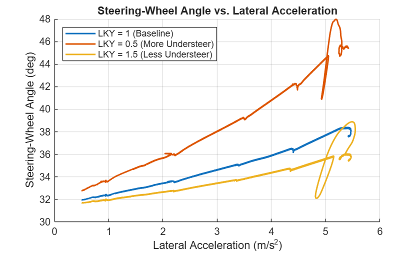
The plot shows three curves. The baseline (LKY = 1) falls between the two extremes. With LKY = 0.5, the steering angle increases more steeply, confirming greater understeer because reduced tire stiffness requires larger slip angles to generate the same lateral force. With LKY = 1.5, the curve is flatter, indicating less understeer as the stiffer tires generate lateral force at smaller slip angles.
Compare Body Sideslip Angle Response
To assess vehicle stability across the LKY sweep, extract and plot the body sideslip angle versus lateral acceleration. Body sideslip angle indicates the direction of travel relative to the vehicle longitudinal axis. Increasingly negative sideslip angle at high lateral acceleration are indicative of a stronger understeer response.
figure
hold on
for idx = 1:numel(lkyValues)
    logs = get(simOut(idx), "logsout");
    ayTS = logs.get("Lateral acceleration").Values;
    betaTS = logs.get("Sideslip angle").Values;
    ayData = ayTS.Data(:);
    betaData = betaTS.Data(:);
    mask = ayData > 0.5;
    plot(ayData(mask), betaData(mask), Color=colors(idx,:), ...
        LineWidth=1.5, DisplayName=lkyLabels(idx))
end
hold off
xlabel("Lateral Acceleration (m/s^2)")
ylabel("Sideslip Angle (deg)")
title("Sideslip Angle vs. Lateral Acceleration")
legend(Location="southwest")
grid on
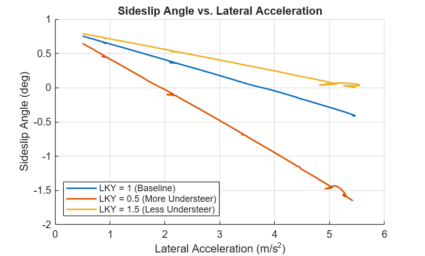
With LKY = 0.5, sideslip grows more negative at high lateral acceleration because the more heavily loaded front tires saturate earlier, rotating the vehicle body away from the turn center. With LKY = 1.5, sideslip remains near zero or positive throughout, because the stiffer tires generate the required level of lateral force at lower slip angle. The baseline LKY = 1 falls between these extremes.
Conclusion
Reducing the LKY scale factor increases understeer (steeper steering angle gradient) and produces larger sideslip excursions as the front tires saturate, while increasing LKY reduces understeer and maintains smaller sideslip angles. You can adapt this workflow to sweep other tire scale factors such as lateral curvature (LCY) or peak lateral friction (LMUY), or combine multiple parameter changes to explore interaction effects on vehicle handling balance.
See Also
Scale Factors | Combined Slip Wheel 2DOF

