Segment and Read Text in Image

Step 1: Detect Candidate Text Regions Using MSER

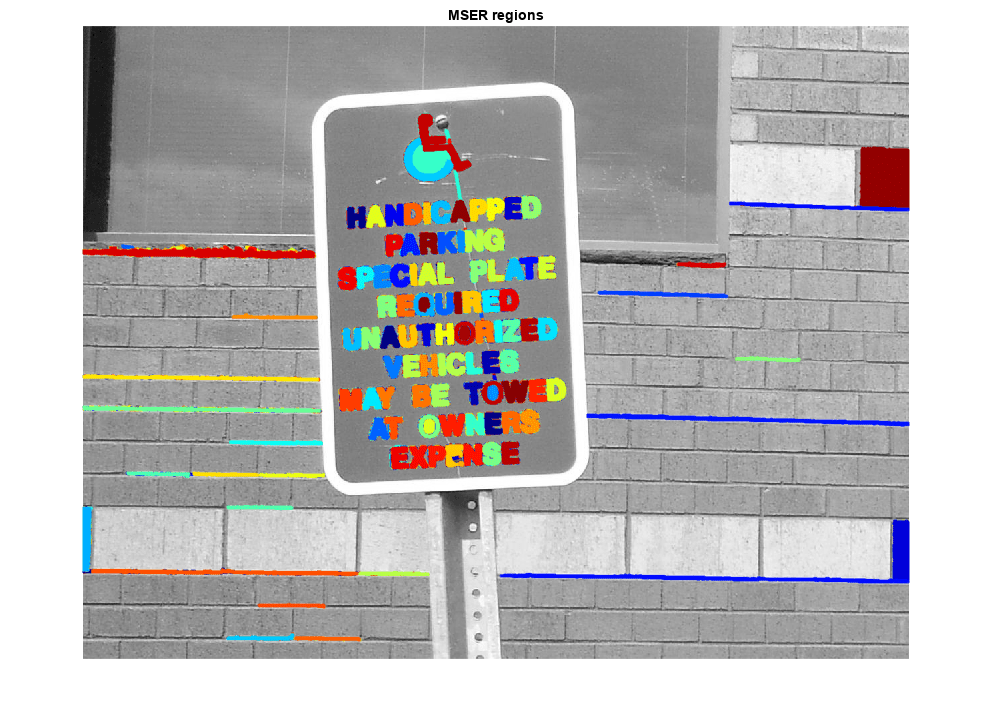
The MSER feature detector works well for finding text regions [1]. It works well for text because the consistent color and high contrast of text leads to stable intensity profiles.

Use the detectMSERFeatures function to find all the regions within the image and plot these results. Notice that there are many non-text regions detected alongside the text.

colorImage = imread("handicapSign.jpg");
I = im2gray(colorImage);

% Detect MSER regions.
[mserRegions, mserConnComp] = detectMSERFeatures(I, ... 
    "RegionAreaRange",[200 8000],"ThresholdDelta",4);

figure
imshow(I)
hold on
plot(mserRegions, "showPixelList", true,"showEllipses",false)
title("MSER regions")
hold off

Step 2: Remove Non-Text Regions Based On Basic Geometric Properties

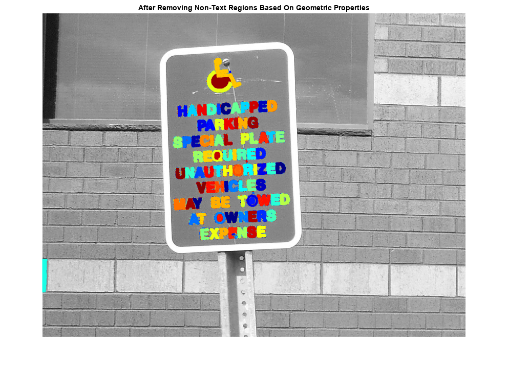
Although the MSER algorithm picks out most of the text, it also detects many other stable regions in the image that are not text. You can use a rule-based approach to remove non-text regions. For example, geometric properties of text can be used to filter out non-text regions using simple thresholds. Alternatively, you can use a machine learning approach to train a text vs. non-text classifier. Typically, a combination of the two approaches produces better results [4]. This example uses a simple rule-based approach to filter non-text regions based on geometric properties.

There are several geometric properties that are good for discriminating between text and non-text regions [2,3], including:

Use regionprops to measure a few of these properties and then remove regions based on their property values.

% Use regionprops to measure MSER properties
mserStats = regionprops(mserConnComp, "BoundingBox", "Eccentricity", ...
    "Solidity", "Extent", "Euler", "Image");

% Compute the aspect ratio using bounding box data.
bbox = vertcat(mserStats.BoundingBox);
w = bbox(:,3);
h = bbox(:,4);
aspectRatio = w./h;

% Threshold the data to determine which regions to remove. These thresholds
% may need to be tuned for other images.
filterIdx = aspectRatio' > 3; 
filterIdx = filterIdx | [mserStats.Eccentricity] > .995 ;
filterIdx = filterIdx | [mserStats.Solidity] < .3;
filterIdx = filterIdx | [mserStats.Extent] < 0.2 | [mserStats.Extent] > 0.9;
filterIdx = filterIdx | [mserStats.EulerNumber] < -4;

% Remove regions
mserStats(filterIdx) = [];
mserRegions(filterIdx) = [];

% Show remaining regions
figure
imshow(I)
hold on
plot(mserRegions, "showPixelList", true,"showEllipses",false)
title("After Removing Non-Text Regions Based On Geometric Properties")
hold off

Step 3: Remove Non-Text Regions Based On Stroke Width Variation

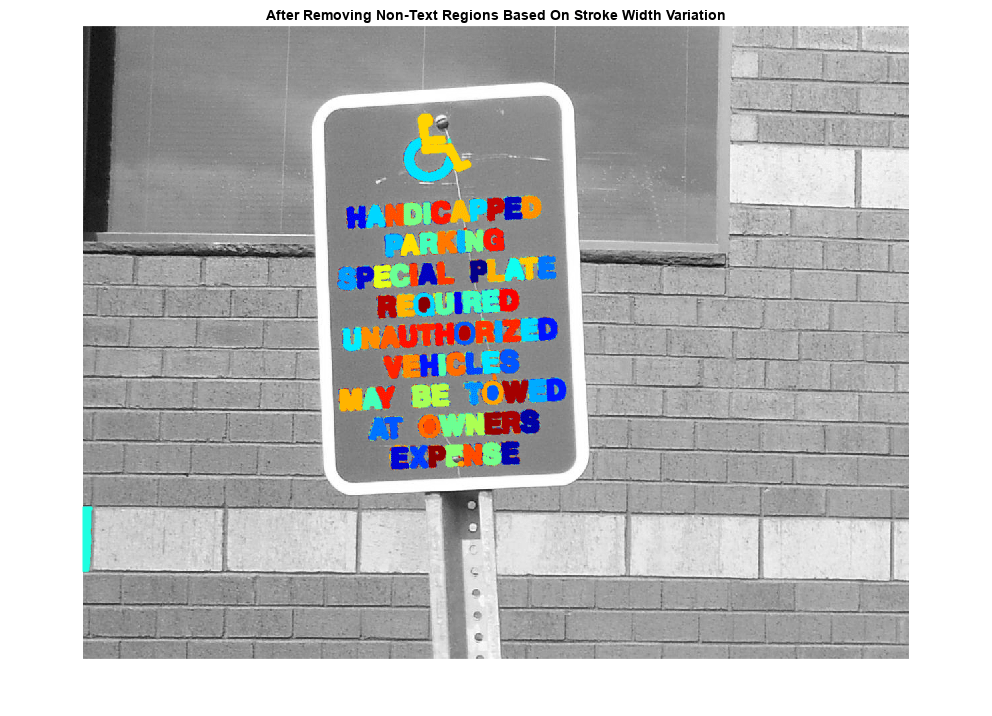
Another common metric used to discriminate between text and non-text is stroke width. Stroke width is a measure of the width of the curves and lines that make up a character. Text regions tend to have little stroke width variation, whereas non-text regions tend to have larger variations.

To help understand how the stroke width can be used to remove non-text regions, estimate the stroke width of one of the detected MSER regions. You can do this by using a distance transform and binary thinning operation [3].

% Get a binary image of the a region, and pad it to avoid boundary effects
% during the stroke width computation.
regionImage = mserStats(6).Image;
regionImage = padarray(regionImage, [1 1]);

% Compute the stroke width image.
distanceImage = bwdist(~regionImage); 
skeletonImage = bwmorph(regionImage, "thin", inf);

strokeWidthImage = distanceImage;
strokeWidthImage(~skeletonImage) = 0;

% Show the region image alongside the stroke width image. 
figure
subplot(1,2,1)
imagesc(regionImage)
title("Region Image")

subplot(1,2,2)
imagesc(strokeWidthImage)
title("Stroke Width Image")

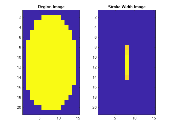
In the images shown above, notice how the stroke width image has very little variation over most of the region. This indicates that the region is more likely to be a text region because the lines and curves that make up the region all have similar widths, which is a common characteristic of human readable text.

In order to use stroke width variation to remove non-text regions using a threshold value, the variation over the entire region must be quantified into a single metric as follows:

% Compute the stroke width variation metric 
strokeWidthValues = distanceImage(skeletonImage);   
strokeWidthMetric = std(strokeWidthValues)/mean(strokeWidthValues);

Then, a threshold can be applied to remove the non-text regions. Note that this threshold value may require tuning for images with different font styles.

% Threshold the stroke width variation metric
strokeWidthThreshold = 0.4;
strokeWidthFilterIdx = strokeWidthMetric > strokeWidthThreshold;

The procedure shown above must be applied separately to each detected MSER region. The following for-loop processes all the regions, and then shows the results of removing the non-text regions using stroke width variation.

% Process the remaining regions
for j = 1:numel(mserStats)
    
    regionImage = mserStats(j).Image;
    regionImage = padarray(regionImage, [1 1], 0);
    
    distanceImage = bwdist(~regionImage);
    skeletonImage = bwmorph(regionImage, "thin", inf);
    
    strokeWidthValues = distanceImage(skeletonImage);
    
    strokeWidthMetric = std(strokeWidthValues)/mean(strokeWidthValues);
    
    strokeWidthFilterIdx(j) = strokeWidthMetric > strokeWidthThreshold;
    
end

% Remove regions based on the stroke width variation
mserRegions(strokeWidthFilterIdx) = [];
mserStats(strokeWidthFilterIdx) = [];

% Show remaining regions
figure
imshow(I)
hold on
plot(mserRegions, "showPixelList", true,"showEllipses",false)
title("After Removing Non-Text Regions Based On Stroke Width Variation")
hold off

Step 4: Merge Text Regions For Final Detection Result

At this point, all the detection results are composed of individual text characters. To use these results for recognition tasks, such as OCR, the individual text characters must be merged into words or text lines. This enables recognition of the actual words in an image, which carry more meaningful information than just the individual characters. For example, recognizing the string 'EXIT' vs. the set of individual characters {'X','E','T','I'}, where the meaning of the word is lost without the correct ordering.

One approach for merging individual text regions into words or text lines is to first find neighboring text regions and then form a bounding box around these regions. To find neighboring regions, expand the bounding boxes computed earlier with regionprops. This makes the bounding boxes of neighboring text regions overlap such that text regions that are part of the same word or text line form a chain of overlapping bounding boxes.

% Get bounding boxes for all the regions
bboxes = vertcat(mserStats.BoundingBox);

% Convert from the [x y width height] bounding box format to the [xmin ymin
% xmax ymax] format for convenience.
xmin = bboxes(:,1);
ymin = bboxes(:,2);
xmax = xmin + bboxes(:,3) - 1;
ymax = ymin + bboxes(:,4) - 1;

% Expand the bounding boxes by a small amount.
expansionAmount = 0.02;
xmin = (1-expansionAmount) * xmin;
ymin = (1-expansionAmount) * ymin;
xmax = (1+expansionAmount) * xmax;
ymax = (1+expansionAmount) * ymax;

% Clip the bounding boxes to be within the image bounds
xmin = max(xmin, 1);
ymin = max(ymin, 1);
xmax = min(xmax, size(I,2));
ymax = min(ymax, size(I,1));

% Show the expanded bounding boxes
expandedBBoxes = [xmin ymin xmax-xmin+1 ymax-ymin+1];
IExpandedBBoxes = insertShape(colorImage,"rectangle",expandedBBoxes,"LineWidth",3);

figure
imshow(IExpandedBBoxes)
title("Expanded Bounding Boxes Text")

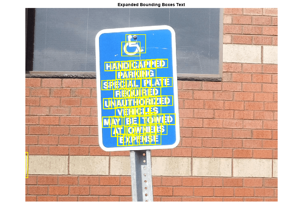
Now, the overlapping bounding boxes can be merged together to form a single bounding box around individual words or text lines. To do this, compute the overlap ratio between all bounding box pairs. This quantifies the distance between all pairs of text regions so that it is possible to find groups of neighboring text regions by looking for non-zero overlap ratios. Once the pair-wise overlap ratios are computed, use a graph to find all the text regions "connected" by a non-zero overlap ratio.

Use the bboxOverlapRatio function to compute the pair-wise overlap ratios for all the expanded bounding boxes, then use graph to find all the connected regions.

% Compute the overlap ratio
overlapRatio = bboxOverlapRatio(expandedBBoxes, expandedBBoxes);

% Set the overlap ratio between a bounding box and itself to zero to
% simplify the graph representation.
n = size(overlapRatio,1); 
overlapRatio(1:n+1:n^2) = 0;

% Create the graph
g = graph(overlapRatio);

% Find the connected text regions within the graph
componentIndices = conncomp(g);

The output of conncomp are indices to the connected text regions to which each bounding box belongs. Use these indices to merge multiple neighboring bounding boxes into a single bounding box by computing the minimum and maximum of the individual bounding boxes that make up each connected component.

% Merge the boxes based on the minimum and maximum dimensions.
xmin = accumarray(componentIndices', xmin, [], @min);
ymin = accumarray(componentIndices', ymin, [], @min);
xmax = accumarray(componentIndices', xmax, [], @max);
ymax = accumarray(componentIndices', ymax, [], @max);

% Compose the merged bounding boxes using the [x y width height] format.
textBBoxes = [xmin ymin xmax-xmin+1 ymax-ymin+1];

Finally, before showing the final detection results, suppress false text detections by removing bounding boxes made up of just one text region. This removes isolated regions that are unlikely to be actual text given that text is usually found in groups (words and sentences).

% Remove bounding boxes that only contain one text region
numRegionsInGroup = histcounts(componentIndices);
textBBoxes(numRegionsInGroup == 1, :) = [];

% Show the final text detection result.
ITextRegion = insertShape(colorImage, "rectangle", textBBoxes,"LineWidth",3);

figure
imshow(ITextRegion)
title("Detected Text")

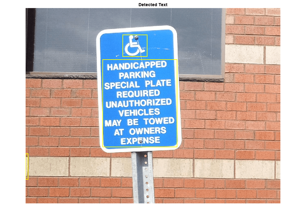
Step 5: Recognize Detected Text Using OCR

After detecting the text regions, use the ocr function to recognize the text within each bounding box. Note that without first finding the text regions, the output of the ocr function would be considerably more noisy.

ocrtxt = ocr(I, textBBoxes);
[ocrtxt.Text]

ans = 
    'HANDICAPPED
     PARKING
     SPECIAL PLATE
     REQUIRED
     UNAUTHORIZED
     VEHICLES
     MAY BE TOWED
     AT OWNERS
     EXPENSE
     
     ie os i uu
     
     '

This example showed you how to detect text in an image using the MSER feature detector to first find candidate text regions, and then it described how to use geometric measurements to remove all the non-text regions. This example code is a good starting point for developing more robust text detection algorithms. Note that without further enhancements this example can produce reasonable results for a variety of other images, for example, posters.jpg or licensePlates.jpg.

References

[1] Chen, Huizhong, et al. "Robust Text Detection in Natural Images with Edge-Enhanced Maximally Stable Extremal Regions." Image Processing (ICIP), 2011 18th IEEE International Conference on. IEEE, 2011.

[2] Gonzalez, Alvaro, et al. "Text location in complex images." Pattern Recognition (ICPR), 2012 21st International Conference on. IEEE, 2012.

[3] Li, Yao, and Huchuan Lu. "Scene text detection via stroke width." Pattern Recognition (ICPR), 2012 21st International Conference on. IEEE, 2012.

[4] Neumann, Lukas, and Jiri Matas. "Real-time scene text localization and recognition." Computer Vision and Pattern Recognition (CVPR), 2012 IEEE Conference on. IEEE, 2012.