Structure from Motion from Two Views
R2026bStructure from motion (SfM) is the process of estimating the 3-D structure of a scene from a set of 2-D images. This example shows you how to estimate the poses of a calibrated camera from two images, reconstruct the 3-D structure of the scene up to an unknown scale factor, and then recover the actual scale factor by detecting an object of a known size.
Overview
This example shows how to reconstruct a 3-D scene from a pair of 2-D images taken with a camera calibrated using the Camera Calibrator app. The algorithm consists of the following steps:
Match a sparse set of points between the two images. There are multiple ways of finding point correspondences between two images. This example detects corners in the first image using the
detectSIFTFeaturesfunction, and tracks them into the second image usingvision.PointTracker. Alternatively you can useextractFeaturesfollowed bymatchFeatures.Estimate the fundamental matrix using
estimateEssentialMatrix.Compute the motion of the camera using the
estrelposefunction.Match a dense set of points between the two images. Re-detect the point using
detectSIFTFeatureswith a reducedContrastThresholdto get more points. Then track the dense points into the second image usingvision.PointTracker.Determine the 3-D locations of the matched points using
triangulateMultiview.Detect an object of a known size. In this scene there is a globe, whose radius is known to be 10cm. Use
pcfitsphereto find the globe in the point cloud.Recover the actual scale, resulting in a metric reconstruction.
Read a Pair of Images
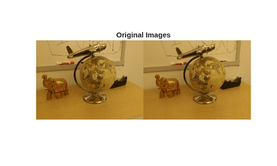
Load a pair of images into the workspace.
imageDir = fullfile(toolboxdir("vision"),"visiondata","upToScaleReconstructionImages");
images = imageDatastore(imageDir);
I1 = readimage(images, 1);
I2 = readimage(images, 2);
figure
imshowpair(I1, I2, 'montage');
title("Original Images");
Load Camera Parameters
This example uses the camera parameters calculated by the Camera Calibrator app. The parameters are stored in the cameraIntrinsics object, and include the camera intrinsics and lens distortion coefficients.
% Load precomputed camera intrinsics
data = load("sfmCameraIntrinsics.mat");
intrinsics = data.intrinsics;
Remove Lens Distortion
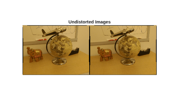
Lens distortion can affect the accuracy of the final reconstruction. You can remove the distortion from each of the images using the undistortImage function. This process straightens the lines that are bent by the radial distortion of the lens.
I1 = undistortImage(I1, intrinsics);
I2 = undistortImage(I2, intrinsics);
figure
imshowpair(I1, I2, "montage");
title("Undistorted Images");
Find Point Correspondences Between the Images
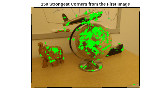
Detect good features to track. If the motion of the camera is not very large, then tracking using the KLT algorithm is a good way to establish point correspondences.
% Detect feature points. Use an ROI to eliminate spurious
% features around the edges of the image.
border = 50;
roi = [border, border, size(I1, 2)- 2*border, size(I1, 1)- 2*border];
imagePoints1 = detectSIFTFeatures(im2gray(I1), ROI=roi, ContrastThreshold=0.015);

% Visualize detected points
figure
imshow(I1);
title("150 Strongest Corners from the First Image");
hold on
plot(selectStrongest(imagePoints1, 1000), ShowScale=false, ShowOrientation=false);
% Create the point tracker
tracker = vision.PointTracker(MaxBidirectionalError=1, NumPyramidLevels=5);

% Initialize the point tracker
imagePoints1 = imagePoints1.Location;
initialize(tracker, imagePoints1, I1);

% Track the points
[imagePoints2, validIdx] = step(tracker, I2);
matchedPoints1 = imagePoints1(validIdx, :);
matchedPoints2 = imagePoints2(validIdx, :);

% Visualize correspondences
figure
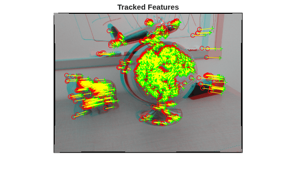
showMatchedFeatures(I1, I2, matchedPoints1, matchedPoints2);
title("Tracked Features");
Estimate the Essential Matrix
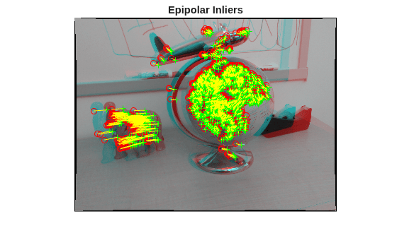
Use the estimateEssentialMatrix function to compute the essential matrix and find the inlier points that meet the epipolar constraint.
% Estimate the fundamental matrix
[E, epipolarInliers] = estimateEssentialMatrix(...
    matchedPoints1, matchedPoints2, intrinsics);

% Find epipolar inliers
inlierPoints1 = matchedPoints1(epipolarInliers, :);
inlierPoints2 = matchedPoints2(epipolarInliers, :);

% Display inlier matches
figure
showMatchedFeatures(I1, I2, inlierPoints1, inlierPoints2);
title("Epipolar Inliers");
Compute the Camera Pose
Compute the location and orientation of the second camera relative to the first one. Note that loc is a translation unit vector, because translation can only be computed up to scale.
relPose = estrelpose(E, intrinsics, inlierPoints1, inlierPoints2);
Reconstruct the 3-D Locations of Matched Points
Re-detect points in the first image using lower ContrastThreshold to get more points. Track the new points into the second image. Estimate the 3-D locations corresponding to the matched points using the triangulate function, which implements the Direct Linear Transformation (DLT) algorithm [1]. Place the origin at the optical center of the camera corresponding to the first image.
% Detect dense feature points.
imagePoints1 = detectSIFTFeatures(im2gray(I1), ROI = roi, ContrastThreshold=0.005);

% Create the point tracker
tracker = vision.PointTracker(MaxBidirectionalError=1, NumPyramidLevels=5);

% Initialize the point tracker
imagePoints1 = imagePoints1.Location;
initialize(tracker, imagePoints1, I1);

% Track the points
[imagePoints2, validIdx] = step(tracker, I2);
matchedPoints1 = imagePoints1(validIdx, :);
matchedPoints2 = imagePoints2(validIdx, :);

% Compute the camera matrices for each position of the camera
% The first camera is at the origin looking along the Z-axis. Thus, its
% transformation is identity.
camMatrix1 = cameraProjection(intrinsics, rigidtform3d);
camMatrix2 = cameraProjection(intrinsics, pose2extr(relPose));

% Compute the 3-D points
points3D = triangulate(matchedPoints1, matchedPoints2, camMatrix1, camMatrix2);

% Get the color of each reconstructed point
numPixels = size(I1, 1) * size(I1, 2);
allColors = reshape(I1, [numPixels, 3]);
colorIdx = sub2ind([size(I1, 1), size(I1, 2)], round(matchedPoints1(:,2)), ...
    round(matchedPoints1(:, 1)));
color = allColors(colorIdx, :);

% Create the point cloud
ptCloud = pointCloud(points3D, Color=color);
Display the 3-D Point Cloud
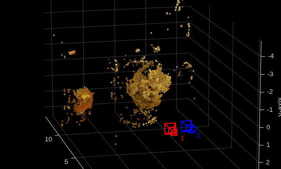
Use the plotCamera function to visualize the locations and orientations of the camera, and the pcshow function to visualize the point cloud.
% Visualize the camera locations and orientations
cameraSize = 0.3;
figure
plotCamera(Size=cameraSize, Color="r", Label="1", Opacity=0);
hold on
grid on
plotCamera(AbsolutePose=relPose, Size=cameraSize, ...
    Color="b", Label="2", Opacity=0);

% Visualize the point cloud
pcshow(ptCloud, VerticalAxis="y", VerticalAxisDir="down", MarkerSize=45);

% Rotate and zoom the plot
camorbit(0, -30);
camzoom(1.5);

% Label the axes
xlabel("x-axis");
ylabel("y-axis");
zlabel("z-axis")

title("Up to Scale Reconstruction of the Scene");
Fit a Sphere to the Point Cloud to Find the Globe
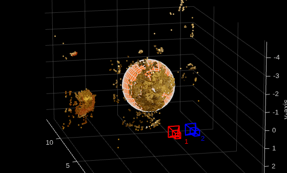
Find the globe in the point cloud by fitting a sphere to the 3-D points using the pcfitsphere function.
% Detect the globe
globe = pcfitsphere(ptCloud, 0.1);

% Display the surface of the globe
plot(globe);
title("Estimated Location and Size of the Globe");
hold off
Metric Reconstruction of the Scene
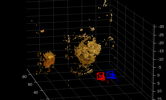
The actual radius of the globe is 10cm. You can now determine the coordinates of the 3-D points in centimeters.
% Determine the scale factor
scaleFactor = 10 / globe.Radius;

% Scale the point cloud
ptCloud = pointCloud(points3D * scaleFactor, Color=color);
relPose.Translation = relPose.Translation * scaleFactor;

% Visualize the point cloud in centimeters
cameraSize = 2;
figure
plotCamera(Size=cameraSize, Color="r", Label="1", Opacity=0);
hold on
grid on
plotCamera(AbsolutePose=relPose, Size=cameraSize, ...
    Color="b", Label="2", Opacity=0);

% Visualize the point cloud
pcshow(ptCloud, VerticalAxis="y", VerticalAxisDir="down", MarkerSize=45);
camorbit(0, -30);
camzoom(1.5);

% Label the axes
xlabel("x-axis (cm)");
ylabel("y-axis (cm)");
zlabel("z-axis (cm)")
title("Metric Reconstruction of the Scene");
Summary
This example showed you how to recover camera motion and reconstruct the 3-D structure of a scene from two images taken with a calibrated camera.
References
[1] Hartley, Richard, and Andrew Zisserman. Multiple View Geometry in Computer Vision. Second Edition. Cambridge, 2000.
See Also
opticalFlowRAFT | detectSIFTFeatures | estimateEssentialMatrix | estrelpose

