What Is Optical Flow?

Optical flow refers to the pattern of apparent motion of objects, surfaces, or edges in a video sequence as observed from a moving or stationary camera. It is a fundamental concept in computer vision, widely used for motion estimation, object tracking, and video analysis. By comparing two consecutive frames of video, you can estimate how fast and in what direction objects are moving.

While optical flow captures apparent motion in an image sequence, the observed motion can arise from different sources. In particular, motion in a video can be caused by moving objects, camera motion, or a combination of both. Understanding this distinction is key to interpreting optical flow results and choosing an appropriate estimation algorithm. Optical flow does not directly distinguish between object motion and camera motion. Instead, it reflects the relative motion between the scene and the camera. Objects that are closer to the camera have greater apparent motion in a series of images than objects that are further away. Except for scenarios in which both the camera and the objects closer to it are stationary, objects that are closer to the camera have greater apparent motion in a series of images than objects that are further away. These scenarios illustrate how different combinations of camera and scene motion affect the observed optical flow in consecutive frames:

Camera is stationary and an object close to the camera is moving — The object appear to move past the camera. For example, a bicycle passing in front of a camera while objects in the background remain stationary.
Camera is moving and objects are stationary — Objects close to the camera appears to move more than distant objects. For example, a stop sign close to a moving camera appears to move past the camera faster than a mountain in the distance.
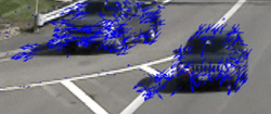
Camera is moving and an object close to the camera is moving — The object close to the camera appears to move fast, while objects further from the camera appear to move more slowly. For example, if a camera is moving in one direction and a car in the foreground is moving in the opposite direction, the car appears to move much faster than stationary trees beyond the car.

Camera Motion and Optical Flow

When the camera moves in a static scene, the observed optical flow is fully explained by the translational and rotational motion of that camera. This relationship shows why optical flow behaves differently for near and far objects, and why some motions are easier to interpret than others. Translational motion produces optical flow that varies with scene depth, whereas rotational motion produces optical flow that is independent of depth.

Consider a camera, of a known focal length f, moving in a static scene with a 3-D translational velocity $(U, V, W)$ and a 3-D angular velocity $(A, B, C)$ , where U and A are along the x-axis, V and B are along the y-axis, and W and C are along the z-axis. The position of each pixel p in image coordinates is denoted as (X, Y). This figure illustrates the translational and rotational velocities of a static scene based on the camera motion:

The optical flow $v$ at a particular pixel location p is the projection of the 3-D motion onto the 2-D image plane. You can express the optical flow vector $v$ as a sum of its translational and rotational components:

$v = v_{r} + v_{t}$

The translational component of optical flow $v_{t}$ is caused by the translational motion of the camera $(U, V, W)$ , and is expressed as:

$v_{t} = (\begin{array}{l} \frac{- f U + x W}{Z} \\ \frac{- f V + y W}{Z} \end{array})$

Observe that the components of the vector $v_{t}$ in the x- and y-directions contain the depth of the scene $Z$ in the denominator. This creates an inverse relationship between translational optical flow and scene depth, causing objects further away from the camera to appear to move less, compared to objects closer to the camera.

The rotational component of optical flow $v_{r}$ is caused by the rotational motion of the camera $(A, B, C)$ , and is expressed as:

$v_{r} = (\begin{array}{l} \frac{A}{f} x y - B f - \frac{B}{f} x^{2} + C y \\ A f + \frac{A}{f} y^{2} - \frac{B}{f} x y - C x \end{array})$

Observe that in the case of camera rotation, the rotational optical flow $(A, B, C)$ is independent of the scene depth $Z$ , and is determined by only the camera rotation and the focal length.

This table summarizes the effects of camera motion on optical flow in static and dynamic scenes. These concepts are useful for gaining a better understanding of the characteristics of optical flow under various kinds of camera motion and object motion.

Scene Motion	Camera Motion	Optical Flow Characteristics
Static scene with no independently moving objects	Translation only	Optical flow is stronger for closer objects and weaker for distant ones, with magnitude inversely proportional to depth [5] [6]. You can use this characteristic for stereo disparity estimation between rectified image pairs. For more information, see Compare RAFT Optical Flow and Semi-Global Matching for Stereo Reconstruction.
	Rotation only	Optical flow is similar for all points regardless of depth. Rotation affects the entire scene uniformly [5] [6].
	Translation and Rotation	Optical flow is a mix of translation and rotation, with magnitude no longer directly indicating depth.
Dynamic scene with independently moving objects	No Translation or Rotation	Optical flow shows the motion of moving objects against a stationary background.
Dynamic scene with independently moving objects	Translation and Rotation	Optical flow in this case is caused by both camera motion, such as the camera being mounted on a forward-moving car, and independently moving objects like other cars or pedestrians. The combination of motions makes it more challenging to distinguish moving objects from the static background, and might require additional logic to separate multiple moving objects from the flow induced by the motion of the camera.

In practice, real-world videos often contain both camera motion and independently moving objects. As a result, the observed optical flow combines multiple motion sources, making interpretation and analysis more challenging. Computer Vision Toolbox™ provides multiple algorithms for estimating optical flow (per-pixel motion) between video frames, and which algorithm you use can significantly affect how well you estimate the object motion.

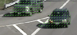
Estimate Optical Flow

Computer Vision Toolbox includes optical flow estimation algorithms based on classic approaches, such as the Horn–Schunck, Lucas–Kanade, and Farneback algorithms, and modern deep learning methods, such as recurrent all-pairs field transforms (RAFT) [4]." Computer Vision Toolbox provides each optical flow algorithm as its own object, each of which returns its estimate as an opticalFlow object that stores the horizontal and vertical components along with the flow magnitude and direction at each pixel. You can visualize the flow vectors using the plot object function and further process the flow for motion analysis.

Although all optical flow algorithms estimate pixel-wise motion, they differ in how they model motion, handle noise, and scale to large displacements. These differences make certain methods better suited for specific applications.

Choose Optical Flow Estimation Algorithm Based on Application

Which optical flow algorithm to use depends on how complex the scene is and how much motion occurs between consecutive frames. Some applications require motion estimates across the entire image, such as motion detection, dense flow estimation, and high-accuracy video analysis, while others only track motion at distinct feature points, such as feature tracking. This table summarizes the strengths, trade-offs, and typical applications of the optical flow methods available in Computer Vision Toolbox.

Optical Flow Method	Strengths	Trade-Offs	Applications
RAFT (Deep Learning)	Suitable for complex scenes and large motions. Captures fine details with dense, accurate flow and pixel correspondences. Offline applications.	Slow and memory-intensive. Requires Deep Learning Toolbox™ and a GPU for efficiency.	Video label propagation, detailed motion analysis, complex scene tracking, disparity from stereo pair estimation, and dense depth estimation from two images. Object: `opticalFlowRAFT`
Farneback	Captures dense, but locally varying flow [3]. Fast, and supports real-time applications.	Less accurate than RAFT in complex scenes. Might fail in uniform texture-less regions.	Motion segmentation, video stabilization, and gesture recognition. Object: `opticalFlowFarneback`
Horn-Schunck (HS)	Captures dense, global flow [2]. Performs well even in low-texture regions. Provides smooth motion fields.	Over-smooths motion boundaries. Less precise for sharp, local motion.	Motion segmentation and video stabilization. Object: `opticalFlowHS`
Lucas-Kanade (LK)	Provides fast, local flow estimation. Captures sparse flow on textured regions. Suitable for small motions.	Assumes constant motion in small windows. Not ideal for large displacements. Computes sparse flow only in regions with strong gradients, which is not ideal for texture-less regions or dense flow at every pixel.	Feature tracking, object tracking, and KLT-based motion analysis. Object: `opticalFlowLK`
Lucas—Kanade Derivative of Gaussian (LKDoG)	Provides fast, local flow estimation. More robust to noise than the LK method, with improved gradient estimation using Gaussian derivatives. Captures sparse flow on textured regions. Suitable for small motions.	Slightly more time-consuming than the LK method. Less sensitive to abrupt motion changes than the LK method. Computes sparse flow only in regions with strong gradients, which is not ideal for texture-less regions or dense flow at every pixel.	Robust point tracking in noisy videos and local motion estimation [1]. Object: `opticalFlowLKDoG`

Applications and Examples of Optical Flow

For more information on how to use various optical flow algorithms, see these examples:

Live Motion Detection Using Optical Flow (Image Acquisition Toolbox) — Perform motion detection and segmentation of a live video using the Horn–Schunck optical flow algorithm.
Automate Labeling of Objects in Video Using RAFT Optical Flow — Automatically transfer polygon ROI annotations between video frames by leveraging RAFT optical flow estimation.
Face Detection and Tracking Using the KLT Algorithm — Automatically detect and track a face using feature points, maintaining robust tracking under head rotation and camera motion
Dense 3-D Reconstruction from Two Views Using RAFT Optical Flow — Estimate relative scene depth from monocular images using optical flow and camera geometry
Compare RAFT Optical Flow and Semi-Global Matching for Stereo Reconstruction — Estimate stereo disparity using RAFT-based optical flow and compare the results with Semi-Global Matching.
Stabilize Video Using Optical Flow — Stabilize jittery video by using optical flow to track pixels across frames and create a smooth camera trajectory.
Activity Recognition from Video and Optical Flow Data Using Deep Learning — Perform activity recognition using a pretrained I3D two-stream CNN and transfer learning with RGB and optical flow video data.
Optical Flow with Parrot Minidrones (Simulink) — Stabilize the Parrot minidrone in space by using downward-facing camera images along with accelerometer and gyroscope data.

References

[1] Barron, J. L., D. J. Fleet, and S. S. Beauchemin. “Performance of Optical Flow Techniques.” International Journal of Computer Vision 12, no. 1 (1994): 43–77. https://doi.org/10.1007/BF01420984.

[2] Horn, Berthold K.P., and Brian G. Schunck. “Determining Optical Flow.” Artificial Intelligence 17, nos. 1–3 (1981): 185–203. https://doi.org/10.1016/0004-3702(81)90024-2.

[3] Farnebäck, Gunnar. “Two-Frame Motion Estimation Based on Polynomial Expansion.” In Image Analysis, edited by Gerhard Goos, Juris Hartmanis, and Jan Van Leeuwen, vol. 2749, edited by Josef Bigun and Tomas Gustavsson. Springer Berlin Heidelberg, 2003. https://doi.org/10.1007/3-540-45103-X_50.

[4] Teed, Zachary, and Jia Deng. "RAFT: Recurrent All-Pairs Field Transforms for Optical Flow." Proceedings of the Thirtieth International Joint Conference on Artificial Intelligence, August 2021, 4839–43. https://doi.org/10.24963/ijcai.2021/662.

[5] Longuet-Higgins, Hugh Christopher, and Kvetoslav Prazdny. "The Interpretation of a Moving Retinal Image." Proceedings of the Royal Society of London. Series B. Biological Sciences 208, no. 1173 (1980): 385-397. https://doi.org/10.1098/rspb.1980.0057.

[6] Bruss, Anna R., and Berthold KP Horn. "Passive Navigation." Computer Vision, Graphics, and Image Processing 21, no. 1 (1983): 3-20. DOI: https://doi.org/10.1016/S0734-189X(83)80026-7.

What Is Optical Flow?

Camera Motion and Optical Flow

Estimate Optical Flow

Choose Optical Flow Estimation Algorithm Based on Application

Applications and Examples of Optical Flow

See Also

Objects

Topics

References