Generate Cartoon Images Using Bilateral Filtering
This example shows how to generate cartoon lines and overlay them onto an image.
Bilateral filtering [1] is used in computer vision systems to filter images while preserving edges and has become ubiquitous in image processing applications. Those applications include denoising while preserving edges, texture and illumination separation for segmentation, and cartooning or image abstraction to enhance edges in a quantized color-reduced image.
Bilateral filtering is simple in concept: each pixel at the center of a neighborhood is replaced by the average of its neighbors. The average is computed using a weighted set of coefficients. The weights are determined by the spatial location in the neighborhood (as in a traditional Gaussian blur filter), and the intensity difference from the center value of the neighborhood.
These two weighting factors are independently controllable by the two standard deviation parameters of the bilateral filter. When the intensity standard deviation is large, the bilateral filter acts more like a Gaussian blur filter, because the intensity Gaussian is less peaked. Conversely, when the intensity standard deviation is smaller, edges in the intensity are preserved or enhanced.
This example model provides a hardware-compatible algorithm. You can generate HDL code from this algorithm, and implement it on a board using an AMD® Zynq® reference design. See Bilateral Filtering with Zynq-Based Hardware (SoC Blockset).
Download Input File
This example uses the potholes2.avi file as an input. The file is approximately 50 MB in size. Download the file from the MathWorks website and unzip the downloaded file.
potholeZipFile = matlab.internal.examples.downloadSupportFile('visionhdl','potholes2.zip');
[outputFolder,~,~] = fileparts(potholeZipFile);
unzip(potholeZipFile,outputFolder);
potholeVideoFile = fullfile(outputFolder,'potholes2');
addpath(potholeVideoFile);
Introduction
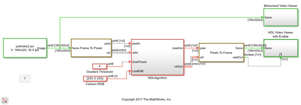
The example model is shown here.
modelname = 'BilateralFilterHDLExample';
open_system(modelname);
set_param(modelname, 'SampleTimeColors', 'on');
set_param(modelname,'SimulationCommand','Update');
set_param(modelname, 'Open', 'on');
set(allchild(0),'Visible', 'off');
Step 1: Establish the Parameter Values
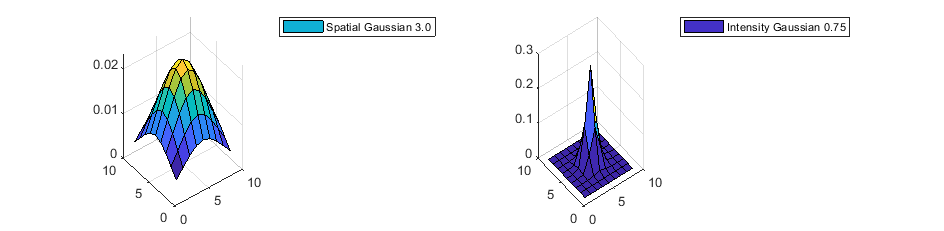
To achieve a modest Gaussian blur of the input, choose a relatively large spatial standard deviation of 3. To give strong emphasis to the edges of the image, choose an intensity standard deviation of 0.75. The intensity Gaussian is built from the image data in the neighborhood, so this plot represents the maximum possible values. Note the small vertical scale on the spatial Gaussian plot.
figure('units','normalized','outerposition',[0 0.5 0.75 0.45]);
subplot(1,2,1);
s1 = surf(fspecial('gaussian',[9 9 ],3));
subplot(1,2,2);
s2 = surf(fspecial('gaussian',[9 9 ],0.75));
legend(s1,'Spatial Gaussian 3.0');
legend(s2,'Intensity Gaussian 0.75');
Fixed-Point Settings
For HDL code generation, you must choose a fixed-point data type for the filter coefficients. The coefficient type should be an unsigned type. For bilateral filtering, the input range is always assumed to be on the interval ![$[0,1]$](../../examples/visionhdl/win64/GenerateCartoonImagesUsingBilateralFilteringExample_eq11732357906191158172.png) . Therefore, a
. Therefore, a uint8 input with a range of values from ![$[0,255]$](../../examples/visionhdl/win64/GenerateCartoonImagesUsingBilateralFilteringExample_eq02766119512029284962.png) are treated as
are treated as ![$\frac{[0,255]}{255} $](../../examples/visionhdl/win64/GenerateCartoonImagesUsingBilateralFilteringExample_eq00857721791321403331.png) . The calculated coefficient values are less than 1. The exact values of the coefficients depend on the neighborhood size and the standard deviations. Larger neighborhoods spread the Gaussian function such that each coefficient value is smaller. A larger standard deviation flattens the Gaussian to produce more uniform values, while a smaller standard deviation produces a peaked response.
. The calculated coefficient values are less than 1. The exact values of the coefficients depend on the neighborhood size and the standard deviations. Larger neighborhoods spread the Gaussian function such that each coefficient value is smaller. A larger standard deviation flattens the Gaussian to produce more uniform values, while a smaller standard deviation produces a peaked response.
If you try a type and the coefficients are quantized such that more than half of the kernel becomes zero for all input, the Bilateral Filter block issues a warning. If all of the coefficients are zero after quantization, the block issues an error.
Step 2: Filter the Intensity Image
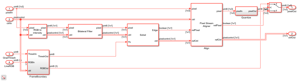
The model converts the incoming RGB image to intensity using the Color Space Converter block. Then the grayscale intensity image is sent to the Bilateral Filter block, which is configured for a 9-by-9 neighborhood and the parameters established previously.
The bilateral filter provides some Gaussian blur but will strongly emphasize larger edges in the image based on the 9-by-9 neighborhood size.
open_system([modelname '/HDLAlgorithm'],'force');
Step 3: Compute Gradient Magnitude
Next, the Edge Detector block, configured for a Sobel algorithm, computes the gradient magnitude. Since the image was prefiltered using a bilateral filter with a fairly large neighborhood, the smaller, less important edges in the image will not be emphasized during edge detection.
The threshold parameter for the edge detection can come from a constant value on the block mask or from a port. The block in this model uses port to allow the threshold to be set dynamically. This threshold value must be computed for your final system, but for now, you can just choose a good value by observing results.
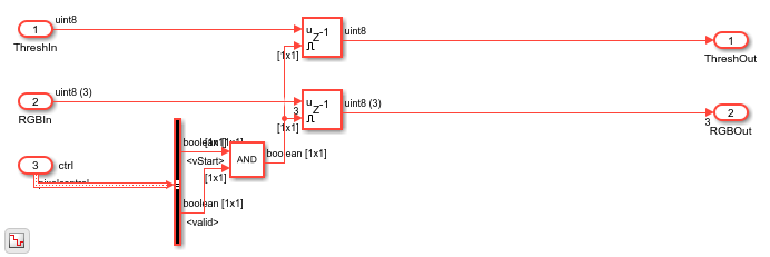
Synchronize the Computed Edges
To overlay the thresholded edges onto the original RGB image, you must realign the two streams. The processing delay of the bilateral filter and edge detector means that the thresholded edge stream and the input RGB pixel stream are not aligned in time.
The Pixel Stream Aligner block brings the streams back together. The RGB pixel stream is connected to the upper pixel input port, and the binary threshold image pixel is connected to the reference input port. The block delays the RGB pixel stream to match the threshold stream.
You must set the number of lines parameter to a value that allows for the delay of both the bilateral filter and the edge detector. The 9-by-9 bilateral filter has a delay of more than 4 lines, while the edge detector has a delay of a bit more than 1 line. For safety, set the Maximum number of lines to 10 for now so that you can try different neighborhood sizes later. Once your design is done, you can determine the actual number of lines of delay by observing the control signal waveforms.
Color Quantization
Color quantization reduces the number of colors in an image to make processing it easier. Color quantization is primarily a clustering problem, because you want to find a single representative color for a cluster of colors in the original image.
For this problem, you can apply many different clustering algorithms, such as k-means or the median cut algorithm. Another common approach is using octrees, which recursively divide the color space into 8 octants. Normally you set a maximum depth of the tree, which controls the recursive subtrees that will be eliminated and therefore represented by one node in the subtree above.
These algorithms require that you know beforehand all of the colors in the original image. In pixel streaming video, the color discovery step introduces an undesirable frame delay. Color quantization is also generally best done in a perceptually uniform color space such as L*a*b. When you cluster colors in RGB space, there is no guarantee that the result will look representative to a human viewer.
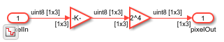
The Quantize subsystem in this model uses a much simpler form of color quantization based on the most significant 4 bits of each 8-bit color component. RGB triples with 8-bit components can represent up to  colors but no single image can use all those colors. Similarly when you reduce the number of bits per color to 4, the image can contain up to
  colors. In practice a 4-bit-per-color image typically contains only several hundred unique colors.
After shifting each color component to the right by 4 bits, the model shifts the result back to the left by 4 bits to maintain the 24-bit RGB format supported by the video viewer. In an HDL system, the next processing steps would pass on only the 4-bit color RGB triples.
open_system([modelname '/HDLAlgorithm/Quantize'],'force');
Overlay the Edges
A switch block overlays the edges on the original image by selecting either the RGB stream or an RGB parameter. The switch is flipped based on the edge-detected binary image. Because cartooning requires strong edges, the model does not use an alpha mixer.
Parameter Synchronization
In addition to the pixel and control signals, two parameters enter the HDLAlgorithm subsystem: the gradient threshold and the line RGB triple for the overlay color. The FrameBoundary subsystem provides run-time control of the threshold and the line color. However, to avoid an output frame with a mix of colors or thresholds, the subsystem registers the parameters only at the start of each frame.
open_system([modelname '/HDLAlgorithm/FrameBoundary'],'force');
Simulation Results
After you run the simulation, you can see that the resulting images from the simulation show bold lines around the detected features in the input video.
HDL Code Generation
To check and generate the HDL code referenced in this example, you must have an HDL Coder™ license.
To generate the HDL code, use the following command.
makehdl('BilateralHDLExample/HDLAlgorithm')
To generate the test bench, use the following command. Note that test bench generation takes a long time due to the large data size. Consider reducing the simulation time before generating the test bench.
makehdltb('BilateralHDLExample/HDLAlgorithm')
The part of the model between the Frame to Pixels and Pixels to Frame blocks can be implemented on an FPGA. The HDLAlgorithm subsystem includes all elements of the bilateral filter, edge detection, and overlay.
Going Further
The bilateral filter in this example is configured to emphasize larger edges while blurring smaller ones. To see the edge detection and overlay without bilateral filtering, right-click the Bilateral Filter block and click the Comment Through button. Then rerun the simulation. The updated results show that many smaller edges are detected and in general, the edges are much noisier.
This model has many parameters you can control, such as the bilateral filter standard deviations, the neighborhood size, and the threshold value. The neighborhood size controls the minimum width of emphasized edges. A smaller neighborhood results in more small edges being highlighted.
You can also control how the output looks by changing the RGB overlay color and the color quantization. Changing the edge detection threshold controls the strength of edges that are overlaid.
To further cartoon the image, you can try adding multiple bilateral filters. With a the right parameters, you can generate a very abstract image that is suitable for a variety of image segmentation algorithms.
Conclusion
This model generated a cartoon image using bilateral filtering and gradient generation. The model overlaid the cartoon lines on a version of the original RGB image that was quantized to a reduced number of colors. This algorithm is suitable for FPGA implementation.
References
[1] Tomasi, C., and R. Manducji. "Bilateral filtering for gray and color images." Sixth International Conference on Computer Vision, 1998.
See Also
Blocks
Functions
imbilatfilt(Image Processing Toolbox) |edge(Image Processing Toolbox)