Stereo Image Rectification
This example shows how to implement stereo image rectification for a calibrated stereo camera pair. The example model is FPGA-hardware compatible and provides real-time performance. This example compares its results with the Computer Vision Toolbox™ rectifyStereoImages function.
Introduction
A stereo camera is a camera system with two or more lenses with a separate image sensor for each lens. They are used for distance estimation, making 3-D pictures, and stereoviews. Camera lenses distort images, and it is difficult to align two cameras to be perfectly parallel. So, the raw images from a pair of stereo cameras must be rectified. Stereo image rectification projects images onto a common image plane in such a way that the corresponding points in the two stereo images have the same row coordinates. This image projection corrects the images to appear as if the two cameras are parallel.
The algorithm used in this example performs distortion removal and alignment correction in a single system.
Stereo Image Rectification Algorithm
The stereo image rectification algorithm uses a reverse mapping technique to map the pixel locations of the output rectified image to the pixels in the input camera image. The diagram shows the four stages of the algorithm.
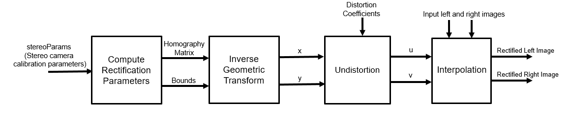
Compute Rectification Parameters: This stage computes rectification parameters from input stereo camera calibration parameters. These calibration parameters include camera intrinsics, rotation matrices, translation matrices, and distortion coefficients (radial and tangential). This stage returns a homography matrix for each camera, and the output bounds. The output bounds are needed to compute the integer pixel coordinates of the output rectified image, and the homography matrices are needed to transform integer pixel coordinates in the output rectified image to corresponding coordinates of the undistorted image.
Inverse Geometric Transform: An inverse geometric transformation translates a point in one image plane onto another image plane. In stereo image rectification, this operation maps integer pixel coordinates in the output rectified image to the corresponding coordinates of the input camera image by using the homography matrix, H. If (p,q) is an integer pixel coordinate in the rectified output image and (x,y) is the corresponding coordinate of the undistorted image, then this equation describes the transformation.
![$$[x \hspace{0.2cm} y \hspace{0.2cm} z]_{3X1} = H^{-1}_{3X3} * [p \hspace{0.2cm} q \hspace{0.2cm} 1]_{3X1} $$](../../examples/visionhdl/win64/StereoImageRectificationHDLExample_eq07976685896271685414.png)
where H is the homography matrix. To convert from homogeneous to cartesian coordinates, x is set to x/z and y is set to y/z.
Undistortion: Lens distortions are optical aberrations which may deform the images. There are two main types of lens distortions: radial and tangential distortions. Radial distortion occurs when light rays bend more near the edges of a lens than they do at its optical center. Tangential distortion occurs when the lens and the image plane are not parallel. For distortion removal, the algorithm maps the coordinates of the undistorted image to the input camera image by using distortion coefficients.
Let (u,v) be the coordinates of the input camera image and (x,y) be the undistorted pixel locations. x and y are normalized from pixel coordinates by translating to the optical center and dividing by the focal length in pixels. The following equations describe the undistortion operation.
 ,
, 
 ,
, 
where  .
.
 ,
,  are radial distortion coefficients and
  ,
,  are tangential distortion coefficients.


Inverse geometric transformation and undistortion both contribute to an overall mapping between the coordinates of the output undistorted rectified image (u,v) and the coordinates of the input camera image.
Interpolation: Interpolation resamples the image intensity values corresponding to the generated coordinates. The example uses bilinear interpolation.
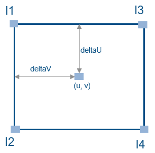
As shown in the diagram, (u,v) is the coordinate of the input pixel generated by the undistortion stage. I1, I2, I3, and I4 are the four neighboring pixels, and deltaU and deltaV are the displacements of the target pixel from its neighboring pixels. This stage computes the weighted average of the four neighboring pixels by using this equation.

HDL Implementation
The figure shows the top-level view of the StereoImageRectificationHDL model. The LeftInputImage and RightInputImage blocks import the stereo left and right images from files. The Frame To Pixels blocks convert these stereo image frames to pixel streams with pixelcontrol buses for input to the HDLStereoImageRectification subsystem. This subsystem performs the inverse geometric transform, undistortion, and interpolation to generate the rectified output pixel values. The Pixels To Frame blocks convert the streams of output pixels back to frames. The LeftImageViewer and RightImageViewer subsystems display the input frames and their corresponding rectified outputs.
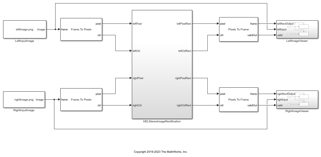
The InitFcn of the example model imports the stereo calibration parameters from a data file and computes the rectification parameters by calling ComputeRectificationParams.m. Alternatively, you can generate your own set of rectification parameters and provide them as mask parameters of the InverseGeometricTransform and Undistortion subsystems.
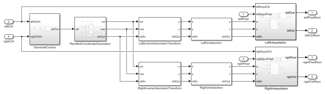
The HDLStereoImageRectification subsystem generates a single pixelcontrol bus from the two input ctrl busses. The RectifiedCoordinateGeneration subsystem generates the row and column pixel coordinates of the output rectified and undistorted image. It uses two HDL counters to generate the row and column coordinates. The InverseGeometricTransform subsystems map these coordinates onto their corresponding row and column coordinates, (x,y), of the distorted image. The Undistortion subsystems map the (x,y) coordinates to its corresponding coordinate (u,v) of the input camera image, using the distortion coefficients and stereo camera intrinsics.
The Interpolation subsystems store the pixel intensities of the input stereo images in a memory and calculate the addresses of the four neighbors of (u,v) required for interpolation. To calculate each rectified output pixel intensity, the subsystem reads the four neighbor pixel values and finds their weighted sum.
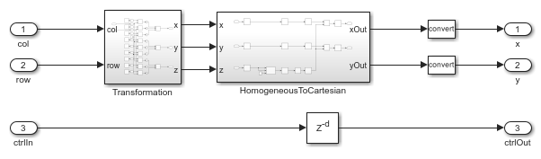
Inverse Geometric Transformation
The HDL implementation of inverse geometric transformation multiplies the coordinates [row col 1] with the inverse homography matrix. The inverse homography matrix (3-by-3) is a masked parameter of the InverseGeometricTransformation subsystem. ComputeRectificationParams.m, called in the InitFcn of the model, generates the homography matrix. The Transformation subsystem implements the matrix multiplication with Product blocks that multiply by each element of the homography matrix. The HomogeneousToCartesian subsystem converts the generated homogeneous coordinates, [x y z] back to the cartesian format, [x y] for further processing. The HomogeneousToCartesian subsystem uses a Reciprocal block configured to use the ShiftAdd architecture, and the UsePipelines parameter is set to 'on'. To see these parameters, right-click the block and in the HDL Coder app section, click HDL Block Properties. Until this stage, the word length was allowed to grow with each operation. After the HomogeneousToCartesian subsystem, the word length of the coordinates is truncated to a size that still ensures precision and accuracy of the generated coordinates.
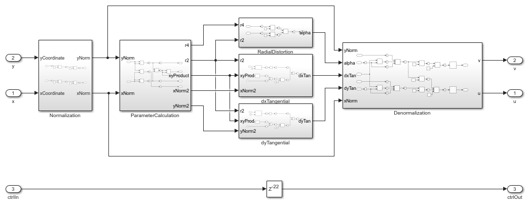
Undistortion
The HDL implementation of Undistortion takes the 3-by-3 camera intrinsic matrix, distortion coefficients [k1 k2 p1 p2], and the reciprocal of fx and fy as masked parameters. ComputeRectificationParams.m, which is called in the InitFcn of the model, generates these parameters. The intrinsic matrix is defined as ![$ \left[ {\begin{array}{ccc} fx & skew & cx\\ 0 & fy & cy\\ 0 & 0 & 1\\ \end{array} } \right] $](../../examples/visionhdl/win64/StereoImageRectificationHDLExample_eq13846193496479939449.png) .
.
The Undistortion subsystem implements the equations mentioned in the Stereo Image Rectification Algorithm section by using Sum, Product, and Shift arithmetic blocks. The word length is allowed to grow with each operation, and then the Denormalization subsystem truncates the word length to a size that still ensures the precision and accuracy of the generated coordinates.
Interpolation
These sections describe the three components inside the Interpolation subsystem.

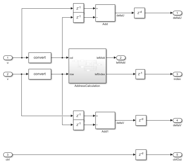
Address Generation
The AddressGeneration subsystem takes the mapped coordinate of the input raw image (u,v) as input. It calculates the displacement deltaU and deltaV of each pixel from its neighboring pixels. It also rounds the coordinates to the nearest integer toward negative infinity.
The AddressCalculation subsystem checks the coordinates against the bounds of the input images. If any coordinate is outside the image dimensions, is capped to the boundary value for further processing. Next, the subsystem calculates the index of the address of each of the four neighborhood pixels in the CacheMemory subsystem. The index represents the column of the cache. The index for each address is determined using the even and odd nature of the incoming column and row coordinates, as determined by the Extract Bits block.
% ==========================
% |Row  || Col  || Index ||
% ==========================
% |Odd  || Odd  ||   1   ||
% |Even || Odd  ||   2   ||
% |Odd  || Even ||   3   ||
% |Even || Even ||   4   ||
% ==========================
The address of the neighborhood pixels is generated using this equation:

where nR is the row coordinate, and nC is the column coordinate.
 ,
,  ,
,  ,
, 
 ,
,  ,
,  ,
, 
Once all the addresses and their corresponding indices are generated, they are vectorized using a Vector Concatenate block. The IndexChangeForMemoryAccess MATLAB Function block rearranges the addresses in increasing order of their indices. This operation ensures the correct fetching of the data from the CacheMemory block. The addresses are then given as an input to the CacheMemory block, and the index, deltaU, and deltaV are passed to the BilinearInterpolation subsystem.
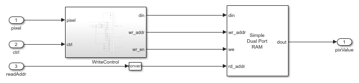
Cache Memory
The CacheMemory subsystem contains a Simple Dual Port RAM block. The input pixels are buffered to form [Line 1 Pixel 1 | Line 2 Pixel 1 | Line 1 Pixel 2 | Line 2 Pixel 2] in the RAM. This configuration enables the algorithm to read all four neighboring pixels in one cycle. The required size of the cache memory is calculated from the offset and displacement parameters in ComputeRectificationParams.m script. The displacement is the sum of maximum deviation and the first row map. The first row map is the maximum value of the input image row coordinate that corresponds to the first row of the output rectified image. Maximum deviation is the greatest difference between the maximum and minimum row coordinates for each row of the input image row map.
The WriteControl subsystem forms vectors of incoming pixels, and vectors of write enables and write addresses. The AddressGeneration subsystem provides a vector of read addresses. The vector of pixels returned from the RAM are passed to the BilinearInterpolation subsystem.
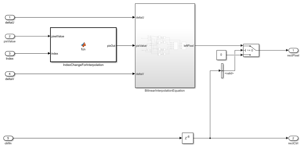
Bilinear Interpolation
The BilinearInterpolation subsystem rearranges the vector of read pixels from the cache to their original indices. Then, the BilinearInterpolationEquation block calculates a weighted sum of the neighborhood pixels by using the bilinear interpolation equation mentioned in the Stereo Image Rectification Algorithm section. The result of the interpolation is the value of the output rectified pixel.
Simulation and Results
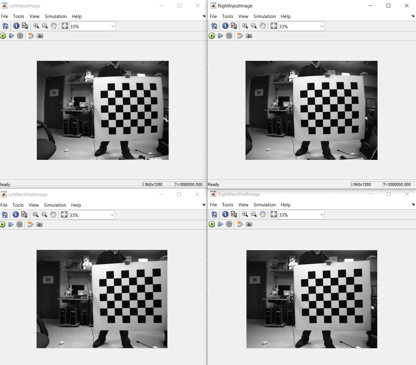
This example uses 960-by-1280 stereo images. The input pixels use the uint8 data type. The example does not provide multipixel support. Due to the large frame sizes used in this example, simulation can take a relatively long time to complete.
The figure shows the left and right input images and the corresponding rectified output images. The results of the StereoImageRectificationHDL model match the output of the rectifyStereoImages function in MATLAB with an error of +/-2.
You can generate HDL code for the HDLStereoImageRectification subsystem. You must have an HDL Coder™ license to generate HDL code. This design was synthesized for the Intel® Arria® 10 GX (115S2F45I1SG) FPGA. The HDL design achieves a clock rate of over 150 MHz. The table shows the resource utilization for the subsystem.
% ===============================================================
% |Model Name              || StereoImageRectificationHDL  ||
% ===============================================================
% |Input Image Resolution  ||         960 x 1280           ||
% |ALM Utilization         ||           10675              ||
% |Total Registers         ||           24487              ||
% |Total RAM Blocks        ||           327                ||
% |Total DSP Blocks        ||           218                ||
% ===============================================================
References
[1] G. Bradski and A. Kaehler, Learning OpenCV : Computer Vision with the OpenCV Library. Sebastopol, CA: O'Reilly, 2008.
See Also
rectifyStereoImages (Computer Vision Toolbox)