Extended and Hierarchical Multiplexing in CAN Messages

R2026b

Since R2026b

Introduction

This example shows how to decode a CAN message that contains signals mutliplexed using extended and hierarchical multiplexing.

Extended and hierarchical multiplexing provide more flexibility than simple multiplexing in organizing signals in a CAN message. For instance, one CAN message can carry more than one multiplexor signal; signals can be multiplexed by multiple multiplexor values; and a signal can be both multiplexed and multiplexor, effectively introducing a signal hierarchy.

Consider the CAN message named PowerTrainTires available in the DBC file CAN_PowerTrainTires.dbc. Leveraging extended multiplexing, the message packs a large number of signals in a payload of 4 bytes. The byte order is Little Endian and the bit counting is LSb first for all signals. The signal hierarchies and bit layout are represented in the following figure.

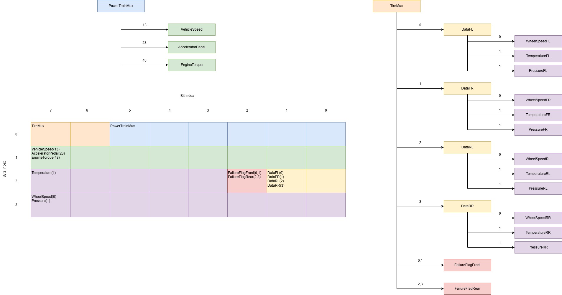
The figure displays signals with overlapping bit locations with the same color. Multiplexor values corresponding to each multiplexed signals are indicated above the arrow connecting a multiplexor to its hierarchy; the same values are repeated in the bit layout, in brackets after the signal names. In the bit layout, the signal names are positioned at their respective MSb.

The message is organized as follows:

Byte 0 store two multiplexors, namely, PowerTrainMux (bits 0-5) and TireMux (bits 6-7); these are the main multiplexor at the top of their respective hierarchy.
The PowerTrainMux signal multiplexes the VehicleSpeed, AcceleratorPedal and EngineTorque signals; these signals all share the same bit locations, that span byte 1.
The TireMux signal multiplexes the four different signals DataFL, DataFR, DataRL, DataRR, which are themselves multiplexors for the data of the front left, front right, rear left and rear right wheels and tires, respectively.
Valid values for the TireMux signal are {0, 1, 2, 3}, mapping to the corresponding wheel position as shown in the hierarchy.
Valid values for DataFL, DataFR, DataRL, DataRR signals are {0, 1}, where 0 maps to the WheelSpeed of the corresponding wheel, while 1 maps to measurements of Pressure and Temperature of its tire.
In the bit layout, the WheelSpeed signals span bits 3 to 7 of byte 2, and the entire byte 3, for a total of 13 bits. In contrast, the Temperature and Pressure signals share those 13 bits, with Temperature spanning bits 3 to 7 of byte 2, while Pressure spanning the entire byte 3.
Bit 2 of byte 2 stores a boolean flag that indicates a combined failure status of the front or rear sensors. Therefore, FailureFlagFront is active only when TireMux is either 0 or 1 (front wheels) while FailureFlagRear is active only when TireMux is either 2 or 3 (rear wheels).

Extended and Hierarchical Multiplexing Information in the CAN Database

The CAN database file is loaded using the canDatabase function. Extract the SignalInfo property in a separate variable.

db = canDatabase("CAN_PowerTrainTires.dbc");
signalInfo = db.MessageInfo.SignalInfo;

Inspect the contents of the structure for the PowerTrainMux signal. In this case, the signal metadata indicate that the signal is a multiplexor, the Multiplexor flag being equal to 1.

signalInfo(strcmp({signalInfo.Name}, 'PowerTrainMux'))

ans = struct with fields:
               Name: 'PowerTrainMux'
            Comment: ''
           StartBit: 0
         SignalSize: 6
          ByteOrder: 'LittleEndian'
             Signed: 0
          ValueType: 'Integer'
              Class: 'uint8'
             Factor: 1
             Offset: 0
            Minimum: 0
            Maximum: 0
              Units: ''
         ValueTable: [0×1 struct]
        Multiplexor: 1
        Multiplexed: 0
      MultiplexMode: 0
    MultiplexorName: ''
            RxNodes: {0×1 cell}
         Attributes: {}
      AttributeInfo: [0×0 struct]

The AcceleratorPedal signal metadata show instead that the signal is multiplexed, the Multiplexed flag being equal to 1; it also shows the name of its multiplexor (in this case, PowerTrainMux) in the MultiplexorName field. The MultiplexMode field carries the value of PowerTrainMux for which AcceleratorPedal is active.

signalInfo(strcmp({signalInfo.Name}, 'AcceleratorPedal'))

ans = struct with fields:
               Name: 'AcceleratorPedal'
            Comment: ''
           StartBit: 8
         SignalSize: 8
          ByteOrder: 'LittleEndian'
             Signed: 0
          ValueType: 'Integer'
              Class: 'uint8'
             Factor: 1
             Offset: 0
            Minimum: 0
            Maximum: 0
              Units: ''
         ValueTable: [0×1 struct]
        Multiplexor: 0
        Multiplexed: 1
      MultiplexMode: 23
    MultiplexorName: 'PowerTrainMux'
            RxNodes: {0×1 cell}
         Attributes: {}
      AttributeInfo: [0×0 struct]

In the case of the FailureFlagFront signal, the MultiplexMode field carries multiple values (in this case, 0 and 1) in a row vector.

signalInfo(strcmp({signalInfo.Name}, 'FailureFlagFront'))

ans = struct with fields:
               Name: 'FailureFlagFront'
            Comment: ''
           StartBit: 18
         SignalSize: 1
          ByteOrder: 'LittleEndian'
             Signed: 0
          ValueType: 'Integer'
              Class: 'uint8'
             Factor: 1
             Offset: 0
            Minimum: 0
            Maximum: 0
              Units: ''
         ValueTable: [0×1 struct]
        Multiplexor: 0
        Multiplexed: 1
      MultiplexMode: [0 1]
    MultiplexorName: 'TireMux'
            RxNodes: {0×1 cell}
         Attributes: {}
      AttributeInfo: [0×0 struct]

The metadata of DataFL show that this signal is both multiplexor and multiplexed, the Multiplexor and Multiplexed flags being both equal to 1.

signalInfo(strcmp({signalInfo.Name}, 'DataFL'))

ans = struct with fields:
               Name: 'DataFL'
            Comment: ''
           StartBit: 16
         SignalSize: 2
          ByteOrder: 'LittleEndian'
             Signed: 0
          ValueType: 'Integer'
              Class: 'uint8'
             Factor: 1
             Offset: 0
            Minimum: 0
            Maximum: 0
              Units: ''
         ValueTable: [0×1 struct]
        Multiplexor: 1
        Multiplexed: 1
      MultiplexMode: 0
    MultiplexorName: 'TireMux'
            RxNodes: {0×1 cell}
         Attributes: {}
      AttributeInfo: [0×0 struct]

Data Decoding and Visualization

The data file testDriveData.blf contains a log of the CAN message PowerTrainTires. Read the log using the blfread function.

data = blfread("testDriveData.blf");

The data is in the form of a CAN message timetable; decode it using the database provided.

msgTT = canMessageTimetable(data{1}, db);

Inspect the first element of the Signals column.

msgTT.Signals{1}

ans = struct with fields:
     FailureFlagRear: NaN
    FailureFlagFront: 0
          PressureRR: NaN
          PressureRL: NaN
          PressureFR: NaN
          PressureFL: NaN
       TemperatureRR: NaN
       TemperatureRL: NaN
       TemperatureFR: NaN
       TemperatureFL: NaN
        WheelSpeedRR: NaN
        WheelSpeedRL: NaN
        WheelSpeedFR: NaN
        WheelSpeedFL: 0
              DataRR: NaN
              DataRL: NaN
              DataFR: NaN
              DataFL: 0
        VehicleSpeed: NaN
        EngineTorque: NaN
    AcceleratorPedal: 0
             TireMux: 0
       PowerTrainMux: 23

The structure contains the values of all the active signals at that time instant; signals that are inactive have values that are effectively missing, and thus are assigned a value of NaN. At the first time instant, the PowerTrainMux and TireMux values indicate that AcceleratorPedal is active as well as the data from the front left wheel; in addition, the DataFL value indicates that the WheelSpeedFL is active; all the other wheel and tire signals are unavailable. Since data from one of the front wheels is available through the WheelSpeedFL signal, also the FailureFlagFront sensor signal is active.

It is convenient to create a signal timetable to facilitate the inspection and visualization of signal values.

sigTT = canSignalTimetable(msgTT);

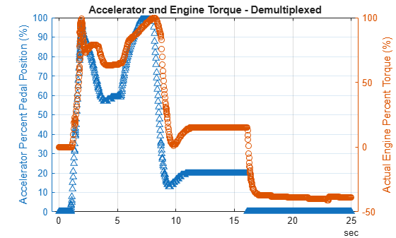
Visualize the AcceleratorPedal and EngineTorque signals after demultiplexing. Note that NaN values are not displayed.

figure;
yyaxis("left");
plot(sigTT.Time, sigTT.AcceleratorPedal, '^');
ylabel("Accelerator Percent Pedal Position (%)")
yyaxis("right");
plot(sigTT.Time, sigTT.EngineTorque, 'o');
grid("on");
ylabel("Actual Engine Percent Torque (%)");
title("Accelerator and Engine Torque - Demultiplexed");

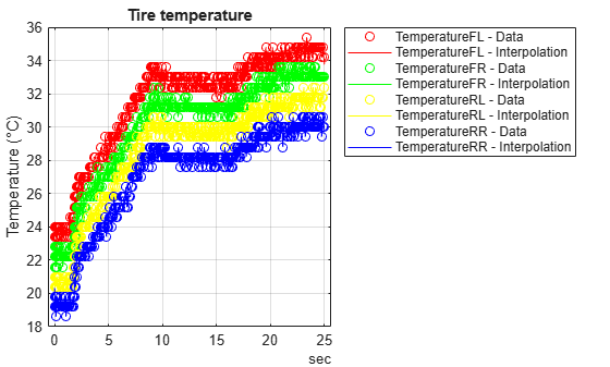
Figure contains an axes object. The axes object with title Accelerator and Engine Torque - Demultiplexed, ylabel Actual Engine Percent Torque (%) contains 2 objects of type line. One or more of the lines displays its values using only markers

Visualize the demultiplexed WheelSpeed, Temperature and Pressure signals for the four wheels. Due to multiplexing, the recorded log has a large number of missing data; markers are used to identify the data, while linear interpolation is used to fill in the gaps.

figure;
plot(sigTT.Time, sigTT.WheelSpeedFL, 'ro');
hold('on');
plot(sigTT.Time, fillmissing(sigTT.WheelSpeedFL, "linear"), 'r-');
plot(sigTT.Time, sigTT.WheelSpeedFR, 'go');
plot(sigTT.Time, fillmissing(sigTT.WheelSpeedFR, "linear"), 'g-');
plot(sigTT.Time, sigTT.WheelSpeedRL, 'yo');
plot(sigTT.Time, fillmissing(sigTT.WheelSpeedRL, "linear"), 'y-');
plot(sigTT.Time, sigTT.WheelSpeedRR, 'bo');
plot(sigTT.Time, fillmissing(sigTT.WheelSpeedRR, "linear"), 'b-');
grid('on');
ylabel("Wheel speed [rad/s]");
legend("WheelSpeedFL - Data", "WheelSpeedFL - Interpolation", ...
    "WheelSpeedFR - Data", "WheelSpeedFR - Interpolation", ...
    "WheelSpeedRL - Data", "WheelSpeedRL - Interpolation", ...
    "WheelSpeedRR - Data", "WheelSpeedRR - Interpolation", "location", "bestoutside");
title("Wheel speed");

figure;
plot(sigTT.Time, sigTT.TemperatureFL, 'ro');
hold('on');
plot(sigTT.Time, fillmissing(sigTT.TemperatureFL, "linear"), 'r-');
plot(sigTT.Time, sigTT.TemperatureFR, 'go');
plot(sigTT.Time, fillmissing(sigTT.TemperatureFR, "linear"), 'g-');
plot(sigTT.Time, sigTT.TemperatureRL, 'yo');
plot(sigTT.Time, fillmissing(sigTT.TemperatureRL, "linear"), 'y-');
plot(sigTT.Time, sigTT.TemperatureRR, 'bo');
plot(sigTT.Time, fillmissing(sigTT.TemperatureRR, "linear"), 'b-');
grid('on');
ylabel("Temperature (°C)");
legend("TemperatureFL - Data", "TemperatureFL - Interpolation", ...
    "TemperatureFR - Data", "TemperatureFR - Interpolation", ...
    "TemperatureRL - Data", "TemperatureRL - Interpolation", ...
    "TemperatureRR - Data", "TemperatureRR - Interpolation", "Location", "bestoutside");
title("Tire temperature");

figure;
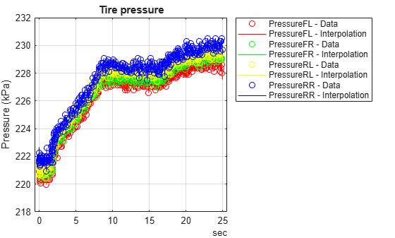
plot(sigTT.Time, sigTT.PressureFL, 'ro');
hold('on');
plot(sigTT.Time, fillmissing(sigTT.PressureFL, "linear"), 'r-');
plot(sigTT.Time, sigTT.PressureFR, 'go');
plot(sigTT.Time, fillmissing(sigTT.PressureFR, "linear"), 'g-');
plot(sigTT.Time, sigTT.PressureRL, 'yo');
plot(sigTT.Time, fillmissing(sigTT.PressureRL, "linear"), 'y-');
plot(sigTT.Time, sigTT.PressureRR, 'bo');
plot(sigTT.Time, fillmissing(sigTT.PressureRR, "linear"), 'b-');
grid('on');
ylabel("Pressure (kPa)");
legend("PressureFL - Data", "PressureFL - Interpolation", ...
    "PressureFR - Data", "PressureFR - Interpolation", ...
    "PressureRL - Data", "PressureRL - Interpolation", ...
    "PressureRR - Data", "PressureRR - Interpolation", "location", "bestoutside");
title("Tire pressure");