Critically-Sampled Discrete Wavelet Transform
Calculating wavelet coefficients at every possible scale is a fair amount of work, and it generates an awful lot of data. What if we choose only a subset of scales and positions at which to make our calculations?
It turns out, rather remarkably, that if we choose scales and positions based on powers of two — so-called dyadic scales and positions — then our analysis will be much more efficient and just as accurate. We obtain such an analysis from the discrete wavelet transform (DWT). For more information on DWT, see Algorithms in the Wavelet Toolbox User's Guide.
An efficient way to implement this scheme using filters was developed in 1988 by Mallat (see [Mal89] in References). The Mallat algorithm is in fact a classical scheme known in the signal processing community as a two-channel subband coder (see page 1 of the book Wavelets and Filter Banks, by Strang and Nguyen [StrN96]).
This very practical filtering algorithm yields a fast wavelet transform — a box into which a signal passes, and out of which wavelet coefficients quickly emerge. Let's examine this in more depth.
One-Stage Filtering: Approximations and Details
For many signals, the low-frequency content is the most important part. It is what gives the signal its identity. The high-frequency content, on the other hand, imparts flavor or nuance. Consider the human voice. If you remove the high-frequency components, the voice sounds different, but you can still tell what's being said. However, if you remove enough of the low-frequency components, you hear gibberish.
In wavelet analysis, we often speak of approximations and details. The approximations are the high-scale, low-frequency components of the signal. The details are the low-scale, high-frequency components.
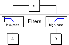
The filtering process, at its most basic level, looks like this.

The original signal, S, passes through two complementary filters and
emerges as two signals.
Unfortunately, if we actually perform this operation on a real digital signal, we wind up with twice as much data as we started with. Suppose, for instance, that the original signal S consists of 1000 samples of data. Then the resulting signals will each have 1000 samples, for a total of 2000.
These signals A and D are interesting, but we get 2000 values instead of the 1000 we
had. There exists a more subtle way to perform the decomposition using wavelets. By looking
carefully at the computation, we may keep only one point out of two in each of the two
2000-length samples to get the complete information. This is the notion of
downsampling. We produce two sequences called cA
and cD.

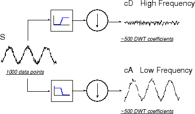
The process on the right, which includes downsampling, produces DWT coefficients.
To gain a better appreciation of this process, let's perform a one-stage discrete wavelet transform of a signal. Our signal will be a pure sinusoid with high-frequency noise added to it.
Here is our schematic diagram with real signals inserted into it.

The MATLAB® code needed to generate s, cD, and
cA is
s
= sin(20.*linspace(0,pi,1000)) + 0.5.*rand(1,1000);
[cA,cD] = dwt(s,'db2');
where db2 is the name of the wavelet we want to use for the
analysis.
Notice that the detail coefficients cD are small and consist mainly
of a high-frequency noise, while the approximation coefficients cA
contain much less noise than does the original signal.
[length(cA) length(cD)]

ans =
   501  501
You may observe that the actual lengths of the detail and approximation coefficient vectors are slightly more than half the length of the original signal. This has to do with the filtering process, which is implemented by convolving the signal with a filter. The convolution “smears” the signal, introducing several extra samples into the result.
Multiple-Level Decomposition
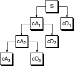
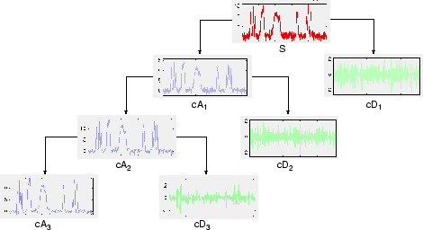
The decomposition process can be iterated, with successive approximations being decomposed in turn, so that one signal is broken down into many lower resolution components. This is called the wavelet decomposition tree.

Looking at a signal's wavelet decomposition tree can yield valuable information.

Number of Levels
Since the analysis process is iterative, in theory it can be continued indefinitely. In reality, the decomposition can proceed only until the individual details consist of a single sample or pixel. In practice, you'll select a suitable number of levels based on the nature of the signal, or on a suitable criterion such as entropy (see Choosing Optimal Decomposition in the Wavelet Toolbox User's Guide).