biorwavf

Return the biorthogonal spline wavelet scaling filters with two vanishing moments.

wname = 'bior2.2';
[RF,DF] = biorwavf(wname)

RF = 1×3

    0.2500    0.5000    0.2500

DF = 1×5

   -0.1250    0.2500    0.7500    0.2500   -0.1250

This example shows how to take analysis and synthesis filters associated with a biorthogonal wavelet and make them compatible with Wavelet Toolbox™. Wavelet Toolbox requires that analysis and synthesis lowpass and highpass filters have equal even length. This example uses the nearly orthogonal biorthogonal wavelets based on the Laplacian pyramid scheme of Burt and Adelson (Table 8.4 on page 283 in [1]). The example also demonstrates how to examine properties of the biorthogonal wavelets.

Define the analysis and synthesis filter coefficients of the biorthogonal wavelet.

Hd = [-1 5 12 5 -1]/20*sqrt(2);
Gd = [3 -15 -73 170 -73 -15 3]/280*sqrt(2);
Hr = [-3 -15 73 170 73 -15 -3]/280*sqrt(2);
Gr = [-1 -5 12 -5 -1]/20*sqrt(2);

Hd and Gd are the lowpass and highpass analysis filters, respectively. Hr and Gr are the lowpass and highpass synthesis filters. They are all finite impulse response (FIR) filters. Confirm the lowpass filter coefficients sum to sqrt(2) and the highpass filter coefficients sum to 0.

sum(Hd)/sqrt(2)

ans = 
1.0000

sum(Hr)/sqrt(2)

ans = 
1.0000

sum(Gd)

ans = 
-1.0061e-16

sum(Gr)

ans = 
-9.7145e-17

The z-transform of an FIR filter $$h$$ is a Laurent polynomial $$h(z)$$ given by $$h(z)=\sum _{k=k_b}^{k_e}{h}_k{z}^{-k}$$. The degree $$|h|$$ of a Laurent polynomial is defined as $$|h|=k_e-k_b$$. Therefore, the length of the filter $$h$$ is $$1+|h|$$. Examine the Laurent expansion of the scaling and wavelet filters.

PHd = laurentPolynomial(Coefficients=Hd,MaxOrder=2)

PHd = 
  laurentPolynomial with properties:

    Coefficients: [-0.0707 0.3536 0.8485 0.3536 -0.0707]
        MaxOrder: 2

PHr = laurentPolynomial(Coefficients=Hr,MaxOrder=3)

PHr = 
  laurentPolynomial with properties:

    Coefficients: [-0.0152 -0.0758 0.3687 0.8586 0.3687 -0.0758 -0.0152]
        MaxOrder: 3

PGd = laurentPolynomial(Coefficients=Gd,MaxOrder=3)

PGd = 
  laurentPolynomial with properties:

    Coefficients: [0.0152 -0.0758 -0.3687 0.8586 -0.3687 -0.0758 0.0152]
        MaxOrder: 3

PGr = laurentPolynomial(Coefficients=Gr,MaxOrder=2)

PGr = 
  laurentPolynomial with properties:

    Coefficients: [-0.0707 -0.3536 0.8485 -0.3536 -0.0707]
        MaxOrder: 2

Since the filters are associated with biorthogonal wavelet, confirm $$PHd(z)PHr(z)+PG(z)PGr(z)=2$$.

PHd*PHr + PGd*PGr

ans = 
  laurentPolynomial with properties:

    Coefficients: 2
        MaxOrder: 0

Wavelet Toolbox™ requires that filters associated with the wavelet have even equal length. To use the Laplacian wavelet filters in the toolbox, you must include the missing powers of the Laurent series as zeros.

The degrees of PHd and PHr are 4 and 6, respectively. The minimum even-length filter that can accommodate the four filters has length 8, which corresponds to a Laurent polynomial of degree 7. The strategy is to prepend and append 0s as evenly as possible so that all filters are of length 8. Prepend 0 to all the filters, and then append two 0s to Hd and Gr.

Hd = [0 Hd 0 0];
Gd = [0 Gd];
Hr = [0 Hr];
Gr = [0 Gr 0 0];

You can examine properties of the biorthogonal wavelets by creating DWT filter banks. Create two custom DWT filter banks using the filters, one for analysis and the other for synthesis. Confirm the filter banks are biorthogonal.

fb = dwtfilterbank('Wavelet','Custom',...
    'CustomScalingFilter',[Hd' Hr'],...
    'CustomWaveletFilter',[Gd' Gr']);

fb2 = dwtfilterbank('Wavelet','Custom',...
    'CustomScalingFilter',[Hd' Hr'],...
    'CustomWaveletFilter',[Gd' Gr'],...
    'FilterType','Synthesis');

fprintf('fb: isOrthogonal = %d\tisBiorthogonal = %d\n',...
    isOrthogonal(fb),isBiorthogonal(fb));

fb: isOrthogonal = 0	isBiorthogonal = 1

fprintf('fb2: isOrthogonal = %d\tisBiorthogonal = %d\n',...
    isOrthogonal(fb2),isBiorthogonal(fb2));

fb2: isOrthogonal = 0	isBiorthogonal = 1

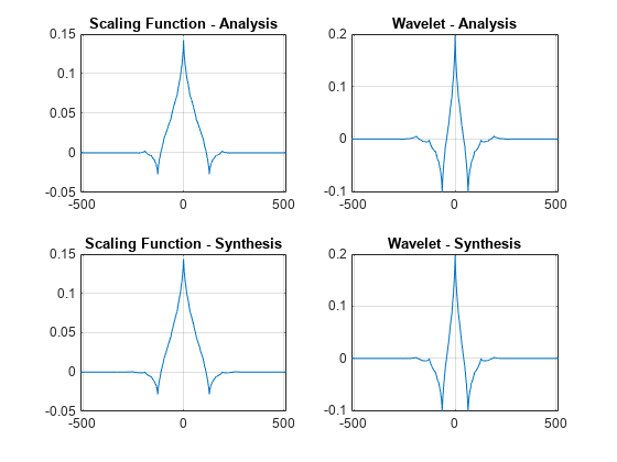
Plot the scaling and wavelet functions associated with the filter banks at the coarsest scale.

[phi,t] = scalingfunctions(fb);
[psi,~] = wavelets(fb);
[phi2,~] = scalingfunctions(fb2);
[psi2,~] = wavelets(fb2);
subplot(2,2,1)
plot(t,phi(end,:))
grid on
title('Scaling Function - Analysis')
subplot(2,2,2)
plot(t,psi(end,:))
grid on
title('Wavelet - Analysis')
subplot(2,2,3)
plot(t,phi2(end,:))
grid on
title('Scaling Function - Synthesis')
subplot(2,2,4)
plot(t,psi2(end,:))
grid on
title('Wavelet - Synthesis')

Compute the filter bank framebounds.

[analysisLowerBound,analysisUpperBound] = framebounds(fb)

analysisLowerBound = 
0.9505

analysisUpperBound = 
1.0211

[synthesisLowerBound,synthesisUpperBound] = framebounds(fb2)

synthesisLowerBound = 
0.9800

synthesisUpperBound = 
1.0528