Main Content

cmddenoise

Interval-dependent denoising

Description

sigden = cmddenoise(sig,wname,level) returns the denoised signal, sigden, obtained from an interval-dependent denoising of the signal, sig, using the orthogonal or biorthogonal wavelet and scaling filters, wname. cmddenoise thresholds the wavelet (detail) coefficients down to level, level, and reconstructs a signal approximation using the modified detail coefficients. cmddenoise partitions the signal into intervals based on variance change points in the first level detail coefficients and thresholds each interval separately. The location and number of variance change points are automatically selected using a penalized contrast function [2]. The minimum delay between change points is 10 samples. Thresholds are obtained using a minimax threshold rule and soft thresholding is used to modify the wavelet coefficients [1].

example

sigden = cmddenoise(sig,wname,level,sorh) returns the denoised signal, sigden, using the thresholding method, sorh, to modify the wavelet coefficients. Valid choices for sorh are 's' for soft thresholding or 'h' for hard thresholding.

example

sigden = cmddenoise(sig,wname,level,sorh,nb_inter) returns the denoised signal, sigden, with the number of denoising intervals as a positive integer between 1 and 6: 1≤ nb_inter ≤6. For nb_inter ≥ 2, cmddenoise estimates the location of the change points with a contrast function [2].

example

sigden = cmddenoise(sig,wname,level,sorh,nb_inter,thrParamsIn) returns the denoised signal, sigden, with the denoising intervals and corresponding thresholds specified as a cell array of matrices with length equal to level. Each element of the cell array contains the interval and threshold information for the corresponding level of the wavelet transform. The elements of thrParamsIn are N-by-3 matrices with N equal to the number of intervals. The 1st and 2nd columns contain the beginning and ending indices of the intervals and the 3rd column contains the corresponding threshold value. If you specify thrParamsIn, cmddenoise ignores the value of nb_inter.

example

[sigden,coefs] = cmddenoise(___) returns the approximation (scaling) and detail (wavelet) coefficients, coefs. The organization of coefs is identical to the structure returned by wavedec. This syntax can include any of the input arguments used in previous syntaxes.

example

[sigden,coefs,thrParamsOut] = cmddenoise(___) returns a cell array, thrParamsOut, with length equal to level. Each element of thrParamsOut is an N-by-3 matrix. The row dimension of the matrix elements is the number of intervals and is determined by the value of the input arguments. Each row of the matrix contains the beginning and end points (indices) of the thresholded interval and the corresponding threshold value.

example

[sigden,coefs,thrParamsOut,int_DepThr_Cell] = cmddenoise(sig,wname,level,sorh,nb_inter) returns a cell array, int_DepThr_Cell, with length equal to 6. int_DepThr_Cell contains interval and threshold information assuming the number of change points ranges from 0 to 5. The N-th element of int_DepThr_Cell is a N-by-3 matrix containing the interval information assuming N-1 change points. Each row of the matrix contains the beginning and end points (indices) of the thresholded interval and the corresponding threshold value. Attempting to output int_DepThr_Cell if you use the input argument, thrParamsIn, results in an error.

example

[sigden,coefs,thrParamsOut,int_DepThr_Cell,BestNbofInt] = cmddenoise(sig,wname,level,sorh,nb_inter) returns the optimal number of signal intervals based on the estimated variance change points in the level-1 detail coefficients. To estimate the number of change points, cmddenoise assumes the total number is less than or equal to 6 and uses a penalized contrast [2]. Attempting to output BestNbofInt if you use the input argument, thrParamsIn, results in an error.

example

Examples

collapse all

Load the noisy blocks signal, nblocr1.mat. The signal consists of a piecewise constant signal in additive white Gaussian noise. The variance of the additive noise differs in three disjoint intervals.

load nblocr1;

Apply interval-dependent denoising down to level 4 using the Haar wavelet. |cmddenoise automatically determines the optimal number and locations of the variance change points. Plot the denoised and original signal for comparison.

sigden = cmddenoise(nblocr1,'db1',4);
plot(nblocr1);
hold on;
plot(sigden,'r','linewidth',2);
axis tight;

Figure contains an axes object. The axes object contains 2 objects of type line.

Load the noisy blocks signal, nblocr1.mat. The signal consists of a piecewise constant signal in additive white Gaussian noise. The variance of the additive noise differs in three disjoint intervals.

load nblocr1;

Apply interval-dependent denoising down to level 4 using the Haar wavelet and a hard thresholding rule. cmddenoise automatically determines the optimal number and locations of the intervals. Plot the original and denoised signals.

sorh = 'h';
sigden = cmddenoise(nblocr1,'db1',4,sorh);
plot(nblocr1);
hold on;
plot(sigden,'r','linewidth',2);
axis tight;
legend('Original Signal','Denoised Signal','Location','NorthWest');

Figure contains an axes object. The axes object contains 2 objects of type line. These objects represent Original Signal, Denoised Signal.

Create a signal sampled at 1 kHz. The signal consists of a series of bumps of various widths.

t = [0.1 0.13 0.15 0.23 0.25 0.40 0.44 0.65 0.76 0.78 0.81];
h = [4  -5 3 -4 5  -4.2   2.1   4.3  -3.1   5.1  -4.2];
h  = abs(h);
len = 1000;
w  = 0.01*[0.5 0.5 0.6 1 1 3 1 1 0.5 0.8 0.5];
tt = linspace(0,1,len);
x = zeros(1,len);
for j=1:11
  x = x + ( h(j) ./ (1+ ((tt-t(j))/w(j)).^4));
end

Add white Gaussian noise with different variances to two disjoint segments of the signal. Add zero-mean white Gaussian noise with variance equal to 2 to the signal segment from 0 to 0.3 seconds. Add zero-mean white Gaussian noise with unit variance to the signal segment from 0.3 seconds to 1 second. Set the random number generator to the default settings for reproducible results.

rng default;
nv1 = sqrt(2).*randn(size(tt)).*(tt<=0.3);
nv2 = randn(size(tt)).*(tt>0.3);
xx = x+nv1+nv2;
sigden = cmddenoise(xx,'sym5',5,'s',2);

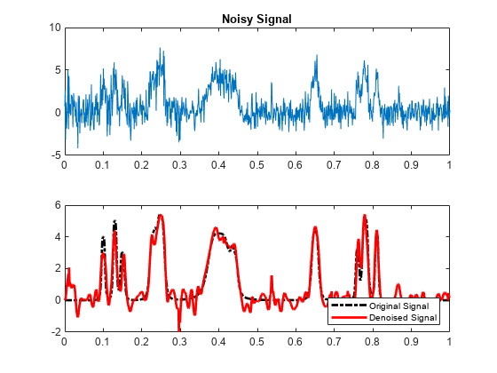
Apply interval-dependent denoising using the Daubechies' least-asymmetric wavelet with 5 vanishing moments down to level 3. Set the number of intervals to 2. Plot the noisy signal, original signal, and denoised signal for comparison.

sigden = cmddenoise(xx,'sym5',3,'s',2);
subplot(211)
plot(tt,xx); title('Noisy Signal');
subplot(212)
plot(tt,x,'k-.','linewidth',2);
hold on;
plot(tt,sigden,'r','linewidth',2);
legend('Original Signal','Denoised Signal','Location','SouthEast');

Figure contains 2 axes objects. Axes object 1 with title Noisy Signal contains an object of type line. Axes object 2 contains 2 objects of type line. These objects represent Original Signal, Denoised Signal.

Load the example signal nbumpr1.mat. The variance of the additive noise differs in three disjoint intervals.

load nbumpr1.mat;

Use a level-5 multiresolution analysis. Create a cell array of length 5 consisting of 3-by-3 matrices. The first two elements of each row contain the beginning and ending indices of the interval and the last element of each row is the corresponding threshold.

wname = 'sym4';
level = 5;
sorh = 's';
thrParamsIn =  {...
    [...
    1     207      1.0482; ...
    207   613      2.5110; ...
    613   1024     1.0031; ...
    ]; ...
    [...
    1    207      1.04824; ...
    207  613      3.8718; ...
    613  1024     1.04824; ...
    ]; ...
    [...
    1    207      1.04824; ...
    207  613      1.99710; ...
    613  1024     1.65613; ...
    ]; ...
    [...
    1    207      1.04824; ...
    207  613      2.09117; ...
    613  1024     1.04824; ...
    ]; ...
    [...
    1    207      1.04824; ...
    207  613      1.78620; ...
    613  102      1.04824; ...
    ]; ...
    };

Denoise the signal using the threshold settings and the Daubechies' least-asymmetric wavelet with 4 vanishing moments. Use a soft thresholding rule. Plot the noisy and denoised signals for comparison.

wname = 'sym4';
level = 5;
sorh = 's';   sigden = cmddenoise(nbumpr1,wname,level,sorh,...
   NaN,thrParamsIn);
plot(nbumpr1); hold on;
plot(sigden,'r','linewidth',2); axis tight;
legend('Noisy Signal','Denoised Signal','Location','NorthEast');

Figure contains an axes object. The axes object contains 2 objects of type line. These objects represent Noisy Signal, Denoised Signal.

Load the example signal nblocr1.mat. Use the Haar wavelet and decompose the signal down to level 2. Obtain the discrete wavelet transform and denoise the signal. Return the wavelet coefficients of the noisy and denoised signals.

load nblocr1.mat;
[sigden,coefs] = cmddenoise(nblocr1,'db1',2);
[C,L] = wavedec(nblocr1,2,'db1');

Plot reconstructions based on the level-2 approximation and level-2 and level-1 detail coefficients for the noisy signal.

app = wrcoef('a',C,L,'db1',2);
subplot(3,1,1);
plot(app); title('Approximation Coefficients');
for nn = 1:2
    det = wrcoef('d',C,L,'db1',nn);
    subplot(3,1,nn+1)
    plot(det); title(['Noisy Wavelet Coefficients - Level '...
          num2str(nn)]);
end

Figure contains 3 axes objects. Axes object 1 with title Approximation Coefficients contains an object of type line. Axes object 2 with title Noisy Wavelet Coefficients - Level 1 contains an object of type line. Axes object 3 with title Noisy Wavelet Coefficients - Level 2 contains an object of type line.

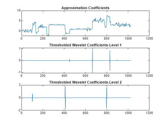
Plot reconstructions based on the approximation and detail coefficients for the denoised signal at the same levels.

figure;
app = wrcoef('a',coefs,L,'db1',2);
subplot(3,1,1);
plot(app); title('Approximation Coefficients');
for nn = 1:2
    det = wrcoef('d',coefs,L,'db1',nn);
    subplot(3,1,nn+1)
    plot(det); 
    title(['Thresholded Wavelet Coefficients-Level '...
         num2str(nn)]);
end

Figure contains 3 axes objects. Axes object 1 with title Approximation Coefficients contains an object of type line. Axes object 2 with title Thresholded Wavelet Coefficients-Level 1 contains an object of type line. Axes object 3 with title Thresholded Wavelet Coefficients-Level 2 contains an object of type line.

The approximation coefficients are identical in the noisy and denoised signal, but most of the detail coefficients in the denoised signal are close to zero.

Create a signal sampled at 1 kHz. The signal consists of a series of bumps of various widths.

t = [0.1 0.13 0.15 0.23 0.25 0.40 0.44 0.65 0.76 0.78 0.81];
h = [4  -5  3  -4 5  -4.2  2.1  4.3  -3.1  5.1  -4.2];
h  = abs(h);
len = 1000;
w  = 0.01*[0.5 0.5 0.6 1 1 3 1 1 0.5 0.8 0.5];
tt = linspace(0,1,len);  x = zeros(1,len);
for j=1:11
  x = x + ( h(j) ./ (1+ ((tt-t(j))/w(j)).^4));
end
plot(tt,x);
title('Original Signal');
hold on;

Figure contains an axes object. The axes object with title Original Signal contains an object of type line.

Add white Gaussian noise with different variances to two disjoint segments of the signal. Add zero-mean white Gaussian noise with variance equal to 2 to the signal segment from 0 to 0.3 seconds. Add zero-mean white Gaussian noise with unit variance to the signal segment from 0.3 seconds to 1 second. Set the random number generator to the default settings for reproducible results.

rng default;
nv1 = sqrt(2).*randn(size(tt)).*(tt<=0.3);
nv2 = randn(size(tt)).*(tt>0.3);
xx = x+nv1+nv2;
plot(tt,xx);
title('Noisy Signal');

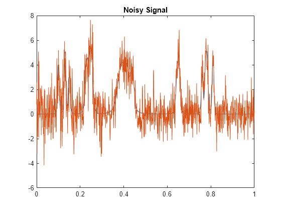
Figure contains an axes object. The axes object with title Noisy Signal contains 2 objects of type line.

Apply interval-dependent denoising using the Daubechies' least- asymmetric wavelet with 4 vanishing moments down to level 5. Automatically choose the number of intervals and output the result.

[sigden,coefs,thrParamsOut] = cmddenoise(xx,'sym4',5);
thrParamsOut{1}
ans = 2×3
103 ×

    0.0010    0.2930    0.0036
    0.2930    1.0000    0.0028

cmdnoise identifies one variance change point in the 1st level detail coefficients defining two intervals. The first interval contains samples 1 to 293. The second interval contains samples 293 to 1000. This is close to the true variance change point, which occurs at sample 299.

Load the example signal, nbumpr1.mat. Partition the signal into 1 to 6 intervals assuming 0 to 5 change points. Compute the thresholds for each interval. Using the Daubechies' least-asymmetric wavelet with 4 vanishing moments return the intervals and corresponding thresholds. Display the results.

load nbumpr1.mat;
[sigden,~,~,int_DepThr_Cell] = cmddenoise(nbumpr1,'sym4',1);
format bank;
disp('          Begin        End          Threshold ');
          Begin        End          Threshold 
cellfun(@disp,int_DepThr_Cell,'UniformOutput',false);
          1.00       1024.00          1.36

          1.00        613.00          1.73
        613.00       1024.00          1.00

          1.00        207.00          1.05
        207.00        613.00          2.51
        613.00       1024.00          1.00

          1.00        207.00          1.05
        207.00        597.00          2.52
        597.00        627.00          1.69
        627.00       1024.00          0.97

          1.00        207.00          1.05
        207.00        613.00          2.51
        613.00        695.00          1.20
        695.00        725.00          0.59
        725.00       1024.00          1.05

          1.00        207.00          1.05
        207.00        597.00          2.52
        597.00        627.00          1.69
        627.00        695.00          1.19
        695.00        725.00          0.59
        725.00       1024.00          1.05

Load the example signal, nbumpr1.mat. The signal has two variance change points, which results in three intervals. Use cmddenoise to detect the number of change points.

load nbumpr1.mat;
[sigden,~,thrParamsOut,~,bestNbofInt] = ...
       cmddenoise(nbumpr1,'sym4',1);
fprintf('Found %d change points.\n',bestNbofInt-1);
Found 2 change points.

Input Arguments

collapse all

Input signal, specified as a 1-D row or column vector. sig is the real-valued input signal for interval-dependent denoising. The elements of sig are assumed to be equally spaced in time or space. If sig contains unequally-sampled data, cmddenoise is not appropriate. Use a lifting transform instead. See mlptdenoise for details.

Data Types: double

Wavelet name, specified as a character vector or string scalar. wname is any valid orthogonal or biorthogonal wavelet. You can use the command: wtype = wavemngr('fields',wname,'type','file'); to determine if the wavelet name is valid to use with cmddenoise. Valid wavelet names return a 1 or 2 for wtype.

Example: 'bior2.2', 'db4', 'sym4'

Data Types: char

Wavelet transform (multiresolution analysis) level, specified as a positive integer. level gives the level of the multiresolution decomposition of the input signal using the decimated 1-D discrete wavelet transform, wavedec.

Data Types: double

Thresholding rule, specified as a character array. sorh is the threshold rule used in the modification of the detail coefficients. Valid choices for sorh are 's' (default) and 'h' for soft and hard thresholding.

Number of intervals, specified as a positive integer less than 7. cmddenoise divides the input signal into nb_inter intervals. cmddenoise determines the location of the nb_inter change points using a contrast function [2]. If you enter NaN for nb_inter, cmddenoise ignores the input. If you use the input argument thrParamsIn, cmddenoise disregards any value you enter for nb_inter.

Data Types: double

Intervals and thresholds by level, specified as a cell array of matrices equal in length to level. Each element of thrParamsIn contains the interval and threshold information for the corresponding level of the multiresolution analysis. The elements of thrParamsIn are N-by-3 matrices with N equal to the number of intervals. The 1st and 2nd columns contain the beginning and ending indices of the intervals and the 3rd column contains the corresponding threshold value. If you specify thrParamsIn, you cannot specify the output arguments int_DepThr_Cell or BestNbofInt.

Data Types: cell

Output Arguments

collapse all

sigden is the denoised version of the input sig. sigden is a 1-D row vector equal in length to sig.

coefs is a row vector of approximation (scaling) and thresholded detail (wavelet) coefficients. The ordering of the approximation and detail coefficients by level in coefs is the same as the output of wavedec. cmddenoise does not apply thresholding to the approximation coefficients.

Data Types: double

thrParamsOut is a cell array of matrices equal in length to level. Each element of the cell array contains the interval and threshold information for the corresponding level of the multiresolution analysis. The elements of thrParamsOut are N-by-3 matrices with N equal to the number of intervals. N is determined by the value of the input arguments. The 1st and 2nd columns contain the beginning and ending indices of the intervals and the 3rd column contains the corresponding threshold value.

Data Types: cell

int_DepThr_Cell contains interval and threshold information assuming the number of change points ranges from 0 to 5. The N-th element of int_DepThr_Cell is a N-by-3 matrix containing the interval information assuming N-1 change points. Each row of the matrix contains the beginning and ending indices of the thresholded interval and the corresponding threshold value. Attempting to output int_DepThr_Cell if you input the number of intervals and thresholds, thrParamsIn, results in an error. int_DepThr_Cell{BestNbofInt} or int_DepThr_Cell{nb_inter} is equal to the matrix elements of thrParamsOut.

Data Types: cell

BestNbofInt is the optimal number of intervals based on estimated change points in the variance of the level-1 detail coefficients. The number and location of the change points are estimated using a penalized contrast method [2]. Attempting to output BestNbofInt if you input the number of intervals and thresholds, thrParamsIn, results in an error.

References

[1] Donoho, D. and Johnstone, I. “Ideal spatial adaptation by wavelet shrinkage”, Biometrika, 1994, 81,3, 425–455.

[2] Lavielle, M. “Detection of multiple changes in a sequence of dependent variables”, Stochastic Processes and their Applications, 1999, 83, 79–102.

Version History

Introduced in R2010a