dddtreecfs

Extract dual-tree/double-density wavelet coefficients or projections

Syntax

out = dddtreecfs(outputtype,wt,outputspec,outputindices)

out = dddtreecfs(outputtype,wt,outputspec,outputindices,'plot')

Description

out = dddtreecfs(outputtype,wt,outputspec,outputindices) extracts the coefficients or subspace projections from the 1-D or 2-D wavelet decomposition, wt. If outputtype equals 'e', out contains wavelet or scaling coefficients. If outputtype equals 'r', out contains wavelet or scaling subspace projections (reconstructions).

example

out = dddtreecfs(outputtype,wt,outputspec,outputindices,'plot') plots the signal or image reconstruction or specified analysis coefficients. You can include the 'plot' option anywhere after the wt input.

example

Examples

collapse all

Reconstruction from 1-D Complex Dual-Tree Wavelet Transform

Open Live Script

Obtain the complex dual-tree wavelet transform of the 1-D noisy Doppler signal. Reconstruct an approximation based on the level-three detail coefficients in multiple ways.

Load the noisy Doppler signal. Obtain the complex dual-tree transform down to level 3.

load noisdopp;
wt = dddtree('cplxdt',noisdopp,3,'dtf1')

wt = struct with fields:
       type: 'cplxdt'
      level: 3
    filters: [1x1 struct]
        cfs: {[1x512x2 double]  [1x256x2 double]  [1x128x2 double]  [1x128x2 double]}

Plot a reconstruction of the original signal based on the level-three detail coefficients with outputspec set to 'scale'.

xr = dddtreecfs('r',wt,'scale',{3},'plot');

Figure CPLXDT contains an axes object. The axes object with title Nodes of Tree: [3], xlabel Reconstructed signal contains an object of type line.

The output xr is a 1-by-1 cell array. Generate the same reconstruction by using 'cumind' and the level-three tree nodes. The first element of each vector in the cell array denotes the level, and the second element denotes the tree. Confirm the reconstructions are identical.

outputindices = {[3 1];[3 2]};
xr2 = dddtreecfs('r',wt,'cumind',outputindices);
max(abs(xr2-xr{1}))

ans = 
0

The output xr2 is the same datatype as the original signal.

Coefficients from 1-D Complex Dual-Tree Wavelet Transform

Open Live Script

Load the noisy Doppler signal. Obtain the complex dual-tree transform down to level 3.

load noisdopp;
wt = dddtree('cplxdt',noisdopp,3,'dtf1')

wt = struct with fields:
       type: 'cplxdt'
      level: 3
    filters: [1×1 struct]
        cfs: {[1×512×2 double]  [1×256×2 double]  [1×128×2 double]  [1×128×2 double]}

Create a cell array of vectors to obtain the second- and third-level detail coefficients from each of the wavelet filter bank trees.

outputindices = {[2 1]; [2 2]; [3 1]; [3 2]};

The first element of each vector in the cell array denotes the level, or stage. The second element denotes the tree.

Extract the detail coefficients.

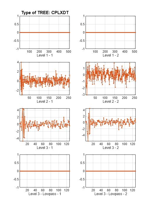
detailCoeffs = dddtreecfs('e',wt,'ind',outputindices,'plot');

The output detailCoeffs is a 1-by-4 cell array. The cell array elements contain the wavelet coefficients corresponding to the elements in outputindices. For example, confirm detailCoeffs{1} contains the level-two detail coefficients from the first tree.

max(abs(wt.cfs{2}(1,:,1)-detailCoeffs{1}))

ans = 0

1-D Complex Dual-Tree Wavelet Transform Structure

Open Live Script

Load the noisy Doppler signal. Obtain the complex dual-tree transform down to level 3.

load noisdopp;
wt = dddtree('cplxdt',noisdopp,3,'dtf1');

Create a cell array of vectors to obtain the second- and third-level detail coefficients from each of the wavelet filter bank trees.

outputindices = {[2 1]; [2 2]; [3 1];[3 2]};

The first element of each vector in the cell array denotes the level, or stage. The second element denotes the tree.

Create a structure array identical to the wt output of dddtree with all the coefficients equal to zero except the second- and third-level detail coefficients.

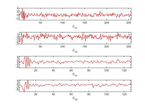
out = dddtreecfs('e',wt,'cumind',outputindices,'plot');

Generate a reconstruction based on the second- and third-level detail coefficients.

xr = idddtree(out);

Generate two reconstructions, based on the second- and third-level detail coefficients. Confirm the sum of the two reconstructions is identical to xr.

xr2 = dddtreecfs('r',wt,'scale',{2;3});
max(abs(xr-(xr2{1}+xr2{2})))

ans = 
4.4409e-16

Extract Diagonal Features from Image

Open Live Script

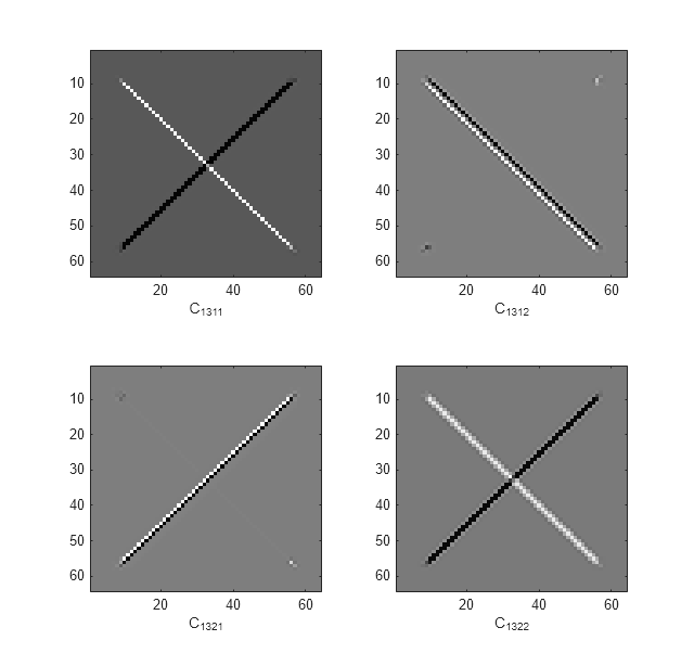
Use the complex dual-tree wavelet transform to isolate diagonal features in an image at +45 and –45 degrees.

Load and display the xbox image.

load xbox
imagesc(xbox)

Figure contains an axes object. The axes object contains an object of type image.

Obtain the complex dual-tree wavelet transform down to level 3.

fdf = dtfilters('FSfarras');
df = dtfilters('qshift10');
wt = dddtree2('cplxdt',xbox,3,fdf,df);

Isolate the +45 and -45 diagonal image features in the level-one wavelet coefficients. Do this by creating a cell array of vectors specifying the tree nodes containing the diagonal details. The first element in the vector specifies the level. The three remaining elements specify the orientation, wavelet tree, and real and imaginary parts, respectively (see dddtree2).

outputindices = {[1 3 1 1];[1 3 1 2];[1 3 2 1];[1 3 2 2]};
out = dddtreecfs('e',wt,'ind',outputindices,'plot');

$Figure CPLXDT contains 4 axes objects. Axes object 1 with xlabel C_{1311} contains an object of type image. Axes object 2 with xlabel C_{1312} contains an object of type image. Axes object 3 with xlabel C_{1321} contains an object of type image. Axes object 4 with xlabel C_{1322} contains an object of type image.$

Distribution of Analysis Coefficients in Wavelet Tree Structure

Open Live Script

This example shows how the analysis coefficients are distributed, depending on the transform, in the tree output of dddtree and dddtree2.

1-D Wavelet Transforms

Load in the noisy Doppler signal. Generate a four-level wavelet decomposition of the signal for each type of transform. Depending on the transform, different dimensions of the coefficient arrays correspond to orientation, wavelet tree, or real and imaginary parts.

Critically Sampled Discrete Wavelet Transform

load noisdopp
wt = dddtree('dwt',noisdopp,4,'sym4')

wt = struct with fields:
       type: 'dwt'
      level: 4
    filters: [1x1 struct]
        cfs: {[1x512 double]  [1x256 double]  [1x128 double]  [1x64 double]  [1x64 double]}

This is the usual nonredundant discrete wavelet transform. The first four elements of wt.cfs are the wavelet coefficients. The fifth element are the scaling coefficients.

Double-Density Wavelet Transform

wt = dddtree('ddt',noisdopp,4,'filters1')

wt = struct with fields:
       type: 'ddt'
      level: 4
    filters: [1x1 struct]
        cfs: {[1x512x2 double]  [1x256x2 double]  [1x128x2 double]  [1x64x2 double]  [1x64 double]}

The third dimension of the 3-D wavelet coefficient arrays corresponds to the tree. The fifth element are the scaling coefficients.

Dual-Tree Complex Wavelet Transform

wt = dddtree('cplxdt',noisdopp,4,'dtf1')

wt = struct with fields:
       type: 'cplxdt'
      level: 4
    filters: [1x1 struct]
        cfs: {[1x512x2 double]  [1x256x2 double]  [1x128x2 double]  [1x64x2 double]  [1x64x2 double]}

The third dimension of all the 3-D arrays in cfs corresponds to the real and imaginary parts. The first four elements of cfs are the wavelet coefficients, and cfs{5} are the scaling coefficients.

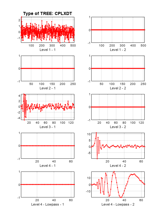
Reconstruct signals from the coefficients at the tree nodes [1 1], [5 2], [3 1], and [4 2]. Plot the signals. The output is a cell array containing the reconstructions. The reconstructions are the same length as the original signal.

outputindices = {[1 1];[5 2];[3 1];[4 2]};
XR = dddtreecfs('r',wt,'plot','ind',outputindices);

$Figure CPLXDT contains 4 axes objects. Axes object 1 with xlabel C_{11} contains an object of type line. Axes object 2 with xlabel C_{52} contains an object of type line. Axes object 3 with xlabel C_{31} contains an object of type line. Axes object 4 with xlabel C_{42} contains an object of type line.$

Extract and plot the coefficients used to reconstruct the signals. The output is a cell array containing the coefficients of respective length: 512, 64, 128, and 64.

XR = dddtreecfs('e',wt,'plot','ind',outputindices);

Now use 'cumind' instead of 'ind'. The output XR is a signal of length 1024 in the first case, and a 'cplxdt' dual-tree in the second one.

XR = dddtreecfs('r',wt,'plot','cumind',outputindices);

Figure CPLXDT contains an axes object. The axes object with title Nodes of Tree: [1 1] , [5 2] , [3 1] , [4 2], xlabel Reconstructed signal contains an object of type line.

XR = dddtreecfs('e',wt,'plot','cumind',outputindices);

Double-Density Dual-Tree Complex Wavelet Transform

wt = dddtree('cplxdddt',noisdopp,4,'dddtf1')

wt = struct with fields:
       type: 'cplxdddt'
      level: 4
    filters: [1x1 struct]
        cfs: {[1x512x2x2 double]  [1x256x2x2 double]  [1x128x2x2 double]  [1x64x2x2 double]  [1x64x2 double]}

The third dimension of the 4-D wavelet coefficient arrays corresponds to the tree. The fourth dimension in the 4-D wavelet coefficient arrays and third dimension in the 3-D scaling coefficients array corresponds to the real and imaginary parts.

2-D Wavelet Transforms

Load in the 256-by-256 mask image. Generate a two-level wavelet decomposition of the image for each type of transform. Observe the dimensions of the output coefficients.

Critically Sampled Discrete Wavelet Transform

load mask
im = X;
wt = dddtree2('dwt',im,3,'sym4')

wt = struct with fields:
       type: 'dwt'
      level: 3
    filters: [1x1 struct]
        cfs: {[128x128x3 double]  [64x64x3 double]  [32x32x3 double]  [32x32 double]}
      sizes: [10x2 double]

This is the usual nonredundant 2-D discrete wavelet transform. The third dimension in the 3-D wavelet coefficient arrays corresponds to the orientation. The scaling coefficients are the last element of cfs.

Real Oriented Dual-Tree Wavelet Transform

wt = dddtree2('realdt',im,3,'dtf1')

wt = struct with fields:
       type: 'realdt'
      level: 3
    filters: [1x1 struct]
        cfs: {[128x128x3x2 double]  [64x64x3x2 double]  [32x32x3x2 double]  [32x32x2 double]}
      sizes: [11x2 double]

The fourth dimension in the 4-D wavelet coefficient arrays and third dimension in the 3-D scaling coefficients array correspond to the tree. The third dimension in the 4-D wavelet coefficient arrays corresponds to orientation.

Complex Oriented Dual-Tree Wavelet Transform

wt = dddtree2('cplxdt',im,3,'dtf1')

wt = struct with fields:
       type: 'cplxdt'
      level: 3
    filters: [1x1 struct]
        cfs: {[5-D double]  [5-D double]  [5-D double]  [32x32x2x2 double]}
      sizes: [11x2 double]

[size(wt.cfs{1});size(wt.cfs{2});size(wt.cfs{3})]

ans = 3×5

   128   128     3     2     2
    64    64     3     2     2
    32    32     3     2     2

The third dimension of the 5-D wavelet coefficient arrays represents the orientation. The fourth dimension in the 5-D arrays and third dimension in the 4-D scaling coefficients array represents the tree. The fifth dimension in the 5-D arrays and fourth dimension in the 4-D array represents the real and imaginary parts.

Double-Density Wavelet Transform

wt = dddtree2('ddt',im,3,'filters1')

wt = struct with fields:
       type: 'ddt'
      level: 3
    filters: [1x1 struct]
        cfs: {[128x128x8 double]  [64x64x8 double]  [32x32x8 double]  [32x32 double]}
      sizes: [26x2 double]

The third dimension in the 3-D wavelet coefficient arrays represents the orientation.

Real Oriented Double-Density Wavelet Transform

wt = dddtree2('realdddt',im,3,'self1')

wt = struct with fields:
       type: 'realdddt'
      level: 3
    filters: [1x1 struct]
        cfs: {[128x128x8x2 double]  [64x64x8x2 double]  [32x32x8x2 double]  [32x32x2 double]}
      sizes: [26x2 double]

The third dimension in the 4-D wavelet coefficient arrays represents the orientation. The fourth dimension in the 4-D arrays and third dimension in the 3-D scaling coefficients array represent the tree.

Complex Oriented Double-Density Wavelet Transform

wt = dddtree2('cplxdddt',im,3,'self1')

wt = struct with fields:
       type: 'cplxdddt'
      level: 3
    filters: [1x1 struct]
        cfs: {[5-D double]  [5-D double]  [5-D double]  [32x32x2x2 double]}
      sizes: [26x2 double]

[size(wt.cfs{1}) ; size(wt.cfs{2}) ; size(wt.cfs{3})]

ans = 3×5

   128   128     8     2     2
    64    64     8     2     2
    32    32     8     2     2

Reconstruct and plot two images based on the second-level detail coefficients and scaling coefficients, respectively.

XR = dddtreecfs('r',wt,'plot','scale',{2;4});

$Figure CPLXDDDT contains 2 axes objects. Axes object 1 with xlabel C_{2} contains an object of type image. Axes object 2 with xlabel C_{4} contains an object of type image.$

The output XR is a cell array containing both 256-by-256 images.

Extract the coefficients used to produce the two images. The output is a cell array containing two dual-tree structures, one for each specified scale.

XR = dddtreecfs('e',wt,'scale',{2;4});
XR{1}

ans = struct with fields:
       type: 'cplxdddt'
      level: 3
    filters: [1x1 struct]
        cfs: {[5-D double]  [5-D double]  [5-D double]  [32x32x2x2 double]}
      sizes: [26x2 double]

XR{2}

ans = struct with fields:
       type: 'cplxdddt'
      level: 3
    filters: [1x1 struct]
        cfs: {[5-D double]  [5-D double]  [5-D double]  [32x32x2x2 double]}
      sizes: [26x2 double]

Confirm the only nonzero coefficients in each structure contained in XR are the level-two wavelet coefficients and scaling coefficients, respectively.

dtInd = 1;
[max(abs(XR{dtInd}.cfs{1}(:)));max(abs(XR{dtInd}.cfs{2}(:)));...
    max(abs(XR{dtInd}.cfs{3}(:)));max(abs(XR{dtInd}.cfs{4}(:)))]

dtInd = 2;
[max(abs(XR{dtInd}.cfs{1}(:)));max(abs(XR{dtInd}.cfs{2}(:)));...
    max(abs(XR{dtInd}.cfs{3}(:)));max(abs(XR{dtInd}.cfs{4}(:)))]

Use 'ind' to reconstruct and display the four images based on the four lowpass components, respectively.

outputindices = {[4 1 1];[4 2 1];[4 1 2];[4 2 2]};
XR = dddtreecfs('r',wt,'plot','ind',outputindices);

$Figure CPLXDDDT contains 4 axes objects. Axes object 1 with xlabel C_{411} contains an object of type image. Axes object 2 with xlabel C_{421} contains an object of type image. Axes object 3 with xlabel C_{412} contains an object of type image. Axes object 4 with xlabel C_{422} contains an object of type image.$

The output XR is a cell array containing the four images. Each image is 256-by-256. Display the coefficients used to reconstruct the images.

XR = dddtreecfs('e',wt,'plot','ind',outputindices);

The output XR is a cell array containing the four lowpass components. Each component is 32-by-32.

Input Arguments

collapse all

`outputtype` — Output type
`'e'` | `'r'`

Output type, specified as 'e' or 'r'. Use 'e' to obtain the scaling or wavelet coefficients. Use 'r' to obtain a projection, or reconstruction, onto the appropriate scaling or wavelet subspace.

`wt` — Wavelet transform
structure

Wavelet transform, specified as a structure. The structure array is the output of dddtree or dddtree2.

`outputspec` — Output specification
`'lowpass'` | `'scale'` | `'ind'` | `'cumind'`

Output specification, specified as one of 'lowpass', 'scale', 'ind', or 'cumind'. The output specifications are defined as follows:

'lowpass' — Outputs the lowpass, or scaling, coefficients or a signal/image approximation based on the scaling coefficients. If you set the output specification to 'lowpass', do not specify outputindices. If the outputtype is 'e', out is a structure array with fields identical to the input structure array wt except that all wavelet (detail) coefficients are equal to zero. If the outputtype is 'r', out is a signal or image approximation based on the scaling coefficients. The signal or image approximation is equal in size to the original input to dddtree or dddtree2.
'scale' — Outputs the coefficients or a signal/image approximation based on the scales specified in outputindices. If the outputtype is 'e', out is a cell array of structure arrays. The fields of the structure arrays in out are identical to the fields of the input structure array wt. The coefficients in the cfs field are all equal to zero except the coefficients corresponding to the scales in outputindices. If the outputtype is 'r', out is a signal or image approximation based on the scales in outputindices. The signal or image approximation is equal in size to the original input to dddtree or dddtree2.
'ind' — Outputs the coefficients or a signal/image approximation based on the tree-position indices specified in outputindices. If the outputtype is 'e', out is a cell array of vectors or matrices containing the coefficients specified by the tree-position indices in outputindices. If the outputtype is 'r', out is a cell array of vectors or matrices containing signal or image approximations based on the corresponding tree-position indices in outputindices.
'cumind' — Outputs the coefficients or a signal/image approximation based on the tree-position indices specified in outputindices. If the outputtype is 'e', out is a structure array. The fields of the structure array are identical to the fields of the input structure array wt. The coefficients in the cfs field are all equal to zero except the coefficients corresponding to the tree positions in outputindices. If the outputtype is 'r', out is a signal or image approximation based on the coefficients corresponding to the tree-position indices in outputindices.

Example: 'ind',{[1 1]; [1 2]}

`outputindices` — Output indices
cell array

Output indices, specified as a cell array with scalar or vector elements. If outputspec equals 'scale', a scalar element selects the corresponding element in the cfs field of wt. If outputspec equals 'ind' or 'cumind', the elements of outputspec are row vectors. The first element of the row vector corresponds to the element in the cfs field of wt. Subsequent elements in the row vector correspond to the indices of the array contained in the cell array element. For a description of the subsequent elements, see Distribution of Analysis Coefficients in Wavelet Tree Structure. For more information, see dddtree and dddtree2.

Example: 'scale',{1;2;3}

Output Arguments

collapse all

`out` — Signal or image reconstruction or coefficients
cell array | structure | vector | matrix

Signal or image reconstruction or coefficients, returned as a vector, matrix, structure array, cell array of vectors or matrices, or cell array of structure arrays. The form of out depends on the value of outputspec and outputindices.

Version History

Introduced in R2013b

dddtreecfs

Syntax

Description

Examples

Reconstruction from 1-D Complex Dual-Tree Wavelet Transform

Coefficients from 1-D Complex Dual-Tree Wavelet Transform

1-D Complex Dual-Tree Wavelet Transform Structure

Extract Diagonal Features from Image

Distribution of Analysis Coefficients in Wavelet Tree Structure

Input Arguments

outputtype — Output type 'e' | 'r'

wt — Wavelet transform structure

outputspec — Output specification 'lowpass' | 'scale' | 'ind' | 'cumind'

outputindices — Output indices cell array

Output Arguments

out — Signal or image reconstruction or coefficients cell array | structure | vector | matrix

Version History

See Also

`outputtype` — Output type
`'e'` | `'r'`

`wt` — Wavelet transform
structure

`outputspec` — Output specification
`'lowpass'` | `'scale'` | `'ind'` | `'cumind'`

`outputindices` — Output indices
cell array

`out` — Signal or image reconstruction or coefficients
cell array | structure | vector | matrix