dwtleader

Multifractal 1-D wavelet leader estimates

Syntax

[dh,h] =
dwtleader(x)

[dh,h,cp]
= dwtleader(x)

[dh,h,cp,tauq]
= dwtleader(x)

[dh,h,cp,tauq,leaders]
= dwtleader(___)

[dh,h,cp,tauq,leaders,structfunc]
= dwtleader(___)

[___]= dwtleader(x,wname)

[___] = dwtleader(___,Name,Value)

Description

[dh,h] = dwtleader(x) returns the singularity spectrum, dh, and the Hölder exponents, h, for the 1-D real-valued data, x. The singularity spectrum and Hölder exponents are estimated for the linearly-spaced moments of the structure functions from –5 to +5.

example

[dh,h,cp] = dwtleader(x) also returns the first three log cumulants, cp of the scaling exponents.

example

[dh,h,cp,tauq] = dwtleader(x) also returns the scaling exponents for the linearly spaced moments from –5 to 5. Wavelet leaders are not defined for the finest scale.

example

[dh,h,cp,tauq,leaders] = dwtleader(___) also returns the wavelet leaders by scale.

[dh,h,cp,tauq,leaders,structfunc] = dwtleader(___) also returns the multiresolution structure functions.

[___]= dwtleader(x,wname) uses the orthogonal or biorthogonal wavelet specified by wname to compute the wavelet leaders and the fractal estimates.

[___] = dwtleader(___,Name,Value) returns the wavelet leaders and other specified outputs with additional options specified by one or more Name,Value pair arguments.

Examples

collapse all

Multifractal Spectrum of Heart-Rate Variability

Open Live Script

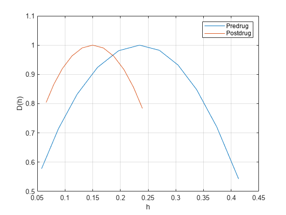
Compare the multifractal spectrum of heart-rate variability data before and after application of a drug that reduces heart dynamics.

load hrvDrug
predrug = hrvDrug(1:4642);
postdrug = hrvDrug(4643:end);
[dhpre,hpre] = dwtleader(predrug);
[dhpost,hpost] = dwtleader(postdrug);
plot(hpre,dhpre,hpost,dhpost)
xlabel('h')
ylabel('D(h)')
grid on
legend('Predrug','Postdrug')

Figure contains an axes object. The axes object with xlabel h, ylabel D(h) contains 2 objects of type line. These objects represent Predrug, Postdrug.

The spread of the Hölder exponent values before drug administration (approximately 0.08 to 0.55) is much larger than the spread of the values afterward (approximately 0.08 to 0.31). This indicates that the heart rate has become more monofractal.

Brownian Noise Singularity Spectrum

Open Live Script

Compute the singularity spectrum and cumulants for a Brownian noise process.

Create the Brownian noise signal.

rng(100);
x = cumsum(randn(2^15,1));

Obtain and plot the singularity spectrum.

[dh,h,cp] = dwtleader(x);
plot(h,dh,'o-','MarkerFaceColor','b') 
grid on
title({'Singularity Spectrum'; ['First Cumulant ' num2str(cp(1))]})

Figure contains an axes object. The axes object with title Singularity Spectrum First Cumulant 0.45539 contains an object of type line.

The small spread in the Hölder exponents (approximately 0.472 to 0.512) indicates that this Brownian noise signal can be characterized by a global Hölder exponent of 0.49875. The theoretical Hölder exponent for Brownian motion is 0.5.

Obtain the cumulants.

cp

cp = 1×3

    0.4554   -0.0121   -0.0000

The first cumulant value is the slope of scaling exponents versus the moments. The second and third cumulants indicate the deviation from linearity. The first cumulant value and near-zero values of the second and third cumulants indicate that the scaling exponents are a linear function of the moments. Therefore, this Brownian motion signal is monofractal.

Multifractal Random Walk Cumulants

Open Live Script

Compute the cumulants for a multifractal random walk. The multifractal random walk is a realization of a random process with a theoretical first cumulant of 0.75 and a second cumulant –0.05. The second cumulant value of –0.05 indicates that the scaling exponents deviate from a linear function with slope 0.75.

Load a random walk signal.

load mrw07505

Obtain and display the first and second cumulants.

[~,~,cp,tauq] = dwtleader(mrw07505);
cp([1 2])

ans = 1×2

    0.7504   -0.0554

For monofractal processes, the scaling exponents are a linear function of the moments. Linearity is indicated by the second and third cumulants being close to zero. In this case, the nonzero second cumulant indicates that the process is multifractal.

Plot the scaling exponents for the q th moments.

plot(-5:5,tauq,'bo--')
title('Estimated Scaling Exponents')
grid on
xlabel('qth Moments')
ylabel('\tau(q)')

Figure contains an axes object. The axes object with title Estimated Scaling Exponents, xlabel qth Moments, ylabel tau (q) contains an object of type line.

The scaling exponents are a nonlinear function of the moments.

Input Arguments

collapse all

`x` — Input signal
vector of real values

Input signal, specified as a 1-D vector of real values. For the default wavelet and minimum regression level, the time series must have at least 248 samples. For nondefault values, the minimum-required data length depends on the wavelet filter and the levels used in the regression model. The wavelet leaders technique works best for data with 8000 or more samples.

Data Types: single | double

`wname` — Wavelet name
`'bior1.5'` (default) | character vector | string scalar

Wavelet name, specified as a character vector or string scalar. wname is a wavelet family short name and filter number recognized by the wavelet manager, wavemngr.

To query valid wavelet family short names, use wavemngr('read'). To determine whether a particular wavelet is orthogonal or biorthogonal, use waveinfo with the wavelet family short name, for example, waveinfo('db'). Alternatively, use wavemngr with the 'type' option, for example, wavemngr('type','fk4'). A returned value of 1 indicates an orthogonal wavelet. A returned value of 2 indicates a biorthogonal wavelet.

Data Types: char | string

Name-Value Arguments

Specify optional pairs of arguments as Name1=Value1,...,NameN=ValueN, where Name is the argument name and Value is the corresponding value. Name-value arguments must appear after other arguments, but the order of the pairs does not matter.

Before R2021a, use commas to separate each name and value, and enclose Name in quotes.

Example: 'MinRegressionLevel',5 sets the minimum regression level to 5.

`RegressionWeight` — Weight option
`'uniform'` (default) | `'scale'`

Weight option to use in the weighted least-squares regression model to determine the singularity spectrum, Hölder exponents, cumulants, and scaling exponents, specified as the comma-separated pair consisting of 'RegressionWeight' and either 'uniform' or 'scale'. The 'uniform' option applies equal weight to each scale. The 'scale' option uses the number of wavelet leaders by scale as weights.

Note

To duplicate the behavior of dwtleader found in releases prior to R2018a, update all instances of dwtleader to include the name-value pair argument 'RegressionWeight' set to 'scale'.

`MinRegressionLevel` — Minimum regression level
`3` (default) | positive integer

Minimum regression level, minlev, specified as the comma-separated pair consisting of 'MinRegressionLevel' and a positive integer greater than or equal to 2. Only levels greater than or equal to the specified minimum level are used in the multifractal estimates. dwtleader requires at least 6 wavelet leaders at the maximum level and two levels to be used in the multifractal estimates. The scale in the discrete wavelet transform corresponding to the minimum level is two^minlev. The smoother the data (that is, the closer the Hölder exponents are to 1), the less likely that reducing the minimum regression level will degrade the results.

`MaxRegressionLevel` — Maximum regression level
positive integer

Maximum regression level, maxlev, specified as a positive integer greater than or equal to minlev + 1. The maximum level uses only levels less than or equal to maxlev in the multifractal estimates. The scale in the discrete wavelet transform corresponding to the maximum level is 2^maxlev. Specify a maximum regression level when you want to restrict the levels used in the regression to a value less than the default level. To determine the number of wavelet leaders by level, use the leaders output argument, or the weights field of the structfunc output argument. The default value is the largest level with at least six wavelet leaders

Output Arguments

collapse all

`dh` — Singularity spectrum
vector

Singularity spectrum, returned as a vector. The singularity spectrum is estimated using structure functions determined for the linearly-spaced moments from –5 to 5. The structure functions are computed based on the wavelet leaders obtained using the biorthogonal spline wavelet filter. The biorthogonal spline wavelet filter that is used has one vanishing moment in the synthesis wavelet and five vanishing moments in the analysis wavelet ('bior1.5'). By default, multifractal estimates are derived from wavelet leaders at a minimum level of 3 and maximum level where there are at least six wavelet leaders.

Data Types: single | double

`h` — Hölder exponent estimates
1-by-11 vector of real scalars

Hölder exponent estimates, returned as a 1-by-11 vector of scalars. Hölder exponents characterize signal regularity. The closer a Hölder exponent is to 1, the closer the function is to differentiable. Conversely, the closer the Hölder exponent is to zero, the closer the function is to discontinuous.

Data Types: single | double

`cp` — Cumulants
vector

Cumulants, returned as a 1–by-3 vector of scalars. The vector contains the first three log cumulants of the scaling exponents. The first cumulant characterizes the linear behavior in the scaling exponents. The second and third cumulants characterize the departure from linearity.

Data Types: single | double

`tauq` — Scaling exponents
column vector

Scaling exponents, returned as a column vector. The exponents are for the linearly-spaced moments from –5 to +5.

Data Types: single | double

`leaders` — Wavelet leaders
cell array

leaders is a cell array with the ith element containing the wavelet leaders at level i+1, or scale 2^{(i +1)}. Wavelet leaders are not defined at level 1.

`structfunc` — Multiresolution structure functions
`struct`

Multiresolution structure functions for the global Hölder exponent estimates, returned as a struct. The structure function for data x is defined as

$S (q, a) = \frac{1}{n_{a}} \sum_{k = 1}^{n_{a}} {| T_{x} (a, k) |}^{q} ≃ a^{ζ (q)},$

where a is the scale, q is the moment, T_x are the wavelet leaders by scale, n_a is the number of wavelet leaders at each scale, and $ζ (q)$ is the scaling exponent. Expanding $ζ (q)$ to a polynomial produces

$ζ (q) = c_{1} q + c_{2} q^{2} / 2 + c 3 q^{3} / 6 + ...$

The scaling exponents can be estimated from the log-cumulants of the wavelet leader coefficients. When $ζ (q)$ is a linear function, the signal is monofractal. When it deviates from linear, the signal is multifractal.

structfunc is a structure array containing the following fields:

Tq — Measurements of the input, x, at various scales. Tq is a matrix of multiresolution quantities that depend jointly on time and scale. Scaling phenomena in x imply a power-law relationship between the moments of Tq and the scale. For dwtleader, the Tq field is an Ns-by-36 matrix, where Ns is the number of scales used in the multifractal estimates. The first 11 columns of Tq are the scaling exponent estimates by scale for each of the qth moments from –5 to 5. The next 11 columns contain the singularity spectrum estimates, dh, for each of the qth moments. Columns 23–33 contain the Hölder exponent estimates, h. The last three columns contain the estimates for the first-order, second-order, and third-order cumulants, respectively.
weights — Weights used in the regression. The weights are the number of wavelet leaders by scale. weights is an Ns-by-1 vector.
logscales — Scales used as predictors in the regression. logscales is an Ns-by-1 vector with the base-2 logarithm of the scales.

Algorithms

Wavelet leaders are derived from the critically sampled discrete wavelet transform (DWT) coefficients. Wavelet leaders offer significant theoretical advantages over wavelet coefficients in the multifractal formalism. Wavelet leaders are time- or space-localized suprema of the absolute value of the discrete wavelet coefficients. The time localization of the suprema requires that the wavelet coefficients are obtained using a compactly supported wavelet. The Hölder exponents, which quantify the local regularity, are determined from these suprema. The singularity spectrum indicates the size of the set of Hölder exponents in the data.

1-D wavelet leaders are defined as

$L_{x} (j, k) = \underset{}{\sup_{λ^{'} \subset 3 λ_{j, k}}} | d_{x} (j, k) |$

where the scales are 2^j, translated to time positions 2^jk. The time neighborhood is $3 λ_{j, k} = λ_{j, k - 1} \cup λ_{j, k} \cup λ_{j, k + 1}$ , where $λ_{j, k} = [k 2^{j}, (k + 1) 2^{j})$ . The time neighborhood is taken over the scale and all finer scales. d_x(j,k) are the wavelet coefficients.

To calculate the wavelet leaders, L_x(j,k):

Compute the wavelet coefficients, d_x(j,k), using the discrete wavelet transform and save the absolute value of each coefficient for each scale. Each finer scale has twice the number of coefficients than the next coarser scale. Each dyadic interval at scale 2^j can be written as a union of two intervals at a finer scale.

$\begin{array}{l} [2^{j} k, 2^{j} (k + 1)) = [2^{j - 1} (2 k), 2^{j - 1} (2 k + 2)) \\ [2^{j - 1} (2 k), 2^{j - 1} (2 k + 2)) = [2^{j - 1} (2 k), 2^{j - 1} (2 k + 1)) \cup [2^{j - 1} (2 k + 1), 2^{j - 1} (2 k + 2)) \end{array}$
Start at the scale that is one level coarser than the finest obtained scale.
Compare the first value to all its finer dyadic intervals and obtain the maximum value.
Go to the next value and compare its value to all of its finer scale values.
Continue comparing the values with their nested values and obtaining the maxima.
From the maximum values obtained for that scale, examine the first three values and obtain the maximum of those neighbors. That maximum value is a leader for that scale.
Continue comparing the maximum values to obtain the other leaders for that scale.
Move to the next coarser scale and repeat the process.

For example, assume that you have these absolute values of the coefficients at these scales:

Starting with the top row, which is the next coarsest level from the finest scale (bottom row), compare each value to its dyadic intervals and obtain the maxima.

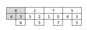
Then, look at the three neighboring values and obtain the maximum. Repeat for the next three neighbors. These maxima, 7 and 7, are the wavelet leaders for this level.

References

[1] Wendt, Herwig, and Patrice Abry. “Multifractality Tests Using Bootstrapped Wavelet Leaders.” IEEE Transactions on Signal Processing 55, no. 10 (October 2007): 4811–20. https://doi.org/10.1109/TSP.2007.896269.

[2] Jaffard, Stéphane, Bruno Lashermes, and Patrice Abry. “Wavelet Leaders in Multifractal Analysis.” In Wavelet Analysis and Applications, edited by Tao Qian, Mang I Vai, and Yuesheng Xu, 201–46. Basel: Birkhäuser Basel, 2007. https://doi.org/10.1007/978-3-7643-7778-6_17.

Extended Capabilities

C/C++ Code Generation
Generate C and C++ code using MATLAB® Coder™.

Usage notes and limitations:

The input wname must be constant.

GPU Arrays
Accelerate code by running on a graphics processing unit (GPU) using Parallel Computing Toolbox™.

The dwtleader function fully supports GPU arrays. To run the function on a GPU, specify the input data as a gpuArray (Parallel Computing Toolbox). For more information, see Run MATLAB Functions on a GPU (Parallel Computing Toolbox).

Version History

Introduced in R2016b

expand all

R2023b: Use `gpuArray` objects

The dwtleader function supports gpuArray objects. You must have Parallel Computing Toolbox™ to use this functionality.

R2023a: Analyze single-precision data and generate C/C++ code

The dwtleader function:

Supports single-precision data.
Supports C/C++ code generation.

You must have MATLAB^® Coder™ to generate C/C++ code.

dwtleader

Syntax

Description

Examples

Multifractal Spectrum of Heart-Rate Variability

Brownian Noise Singularity Spectrum

Multifractal Random Walk Cumulants

Input Arguments

`x` — Input signal
vector of real values

`wname` — Wavelet name
`'bior1.5'` (default) | character vector | string scalar

Name-Value Arguments

`RegressionWeight` — Weight option
`'uniform'` (default) | `'scale'`

`MinRegressionLevel` — Minimum regression level
`3` (default) | positive integer

`MaxRegressionLevel` — Maximum regression level
positive integer

Output Arguments

`dh` — Singularity spectrum
vector

`h` — Hölder exponent estimates
1-by-11 vector of real scalars

`cp` — Cumulants
vector

`tauq` — Scaling exponents
column vector

`leaders` — Wavelet leaders
cell array

`structfunc` — Multiresolution structure functions
`struct`

Algorithms

References

Extended Capabilities

C/C++ Code Generation
Generate C and C++ code using MATLAB® Coder™.

GPU Arrays
Accelerate code by running on a graphics processing unit (GPU) using Parallel Computing Toolbox™.

Version History

R2023b: Use `gpuArray` objects

R2023a: Analyze single-precision data and generate C/C++ code

See Also

Topics

dwtleader

Syntax

Description

Examples

Multifractal Spectrum of Heart-Rate Variability

Brownian Noise Singularity Spectrum

Multifractal Random Walk Cumulants

Input Arguments

x — Input signal vector of real values

wname — Wavelet name 'bior1.5' (default) | character vector | string scalar

Name-Value Arguments

RegressionWeight — Weight option 'uniform' (default) | 'scale'

MinRegressionLevel — Minimum regression level 3 (default) | positive integer

MaxRegressionLevel — Maximum regression level positive integer

Output Arguments

dh — Singularity spectrum vector

h — Hölder exponent estimates 1-by-11 vector of real scalars

cp — Cumulants vector

tauq — Scaling exponents column vector

leaders — Wavelet leaders cell array

structfunc — Multiresolution structure functions struct

Algorithms

References

Extended Capabilities

C/C++ Code Generation Generate C and C++ code using MATLAB® Coder™.

GPU Arrays Accelerate code by running on a graphics processing unit (GPU) using Parallel Computing Toolbox™.

Version History

R2023b: Use gpuArray objects

R2023a: Analyze single-precision data and generate C/C++ code

See Also

Topics

`x` — Input signal
vector of real values

`wname` — Wavelet name
`'bior1.5'` (default) | character vector | string scalar

`RegressionWeight` — Weight option
`'uniform'` (default) | `'scale'`

`MinRegressionLevel` — Minimum regression level
`3` (default) | positive integer

`MaxRegressionLevel` — Maximum regression level
positive integer

`dh` — Singularity spectrum
vector

`h` — Hölder exponent estimates
1-by-11 vector of real scalars

`cp` — Cumulants
vector

`tauq` — Scaling exponents
column vector

`leaders` — Wavelet leaders
cell array

`structfunc` — Multiresolution structure functions
`struct`

C/C++ Code Generation
Generate C and C++ code using MATLAB® Coder™.

GPU Arrays
Accelerate code by running on a graphics processing unit (GPU) using Parallel Computing Toolbox™.

R2023b: Use `gpuArray` objects