lwt2

2-D Lifting wavelet transform

Since R2021b

Syntax

[ll,lh,hl,hh] = lwt2(x)

[___] = lwt2(x,Name=Value)

Description

[ll,lh,hl,hh] = lwt2(x) performs the 2-D lifting wavelet transform (LWT) of the real- or complex-valued matrix x using the db1 wavelet. The function performs the decomposition first along the rows in x and then along the columns. The default decomposition level depends on the size of x. For more information, see Level. The function returns the approximation coefficients at the coarsest scale and the horizontal, vertical, and diagonal detail coefficients by level.

If x is a single-precision input, the numeric type of the coefficients is single precision. Otherwise, the numeric type is double precision.

example

[___] = lwt2(x,Name=Value) specifies options using one or more name-value arguments. For example, lwt2(x,Wavelet="db2",Level=3) performs 2-D LWT using the db2 wavelet and a level 3 decomposition.

example

Examples

collapse all

Lifting Wavelet Transform of 2-D Data

Open Live Script

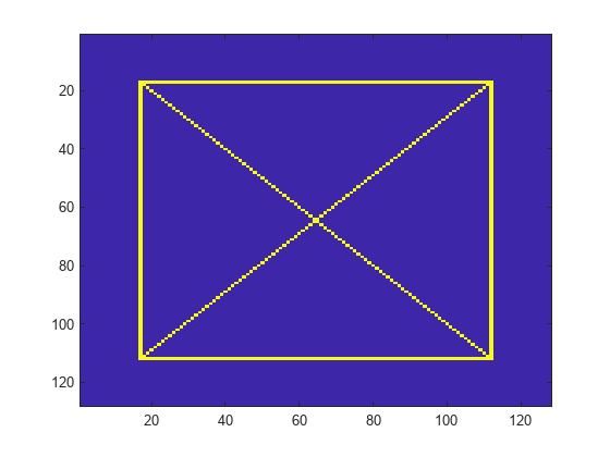
Load and display the xbox image.

load xbox
imagesc(xbox)

Figure contains an axes object. The axes object contains an object of type image.

Obtain the 2-D LWT of the image using default settings.

[ll,lh,hl,hh] = lwt2(xbox);

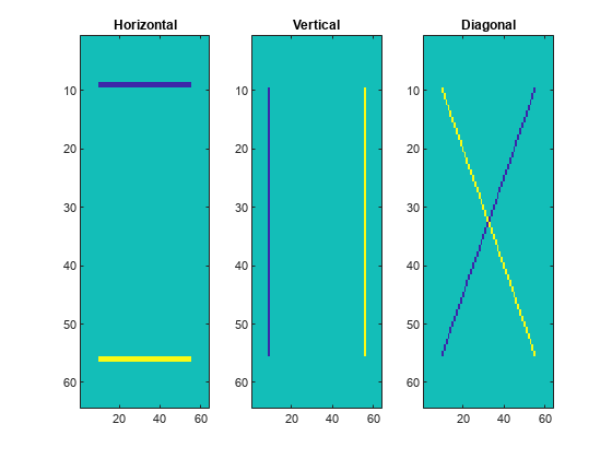
Display the first level detail coefficients.

subplot(1,3,1)
imagesc(lh{1})
title("Horizontal")
subplot(1,3,2)
imagesc(hl{1})
title("Vertical")
subplot(1,3,3)
imagesc(hh{1})
title("Diagonal")

Figure contains 3 axes objects. Axes object 1 with title Horizontal contains an object of type image. Axes object 2 with title Vertical contains an object of type image. Axes object 3 with title Diagonal contains an object of type image.

Lifting Wavelet Transform of RGB Image Using Lifting Scheme

Open Live Script

Load an RGB image. An RGB image is also known as a truecolor image. The image is a 3-D array of type uint8.

x = imread("ngc6543a.jpg");
image(x)

Figure contains an axes object. The axes object contains an object of type image.

Create the lifting scheme associated with the bior3.7 wavelet. Obtain the level 3 LWT of the image using the lifting scheme. Preserve the integer-valued data.

lvl = 3;
lScheme = liftingScheme("Wavelet","bior3.7");
[ll,lh,hl,hh] = lwt2(x,LiftingScheme=lScheme,Level=lvl,Int2Int=true);

Confirm the approximation coefficients are all integer valued. Choose a level and confirm all the detail coefficients at that level are integer valued.

approxDiffs = ll-floor(ll);
max(abs(approxDiffs(:)))

ans = 
0

lev = 2;
horizDiffs = lh{lev}-floor(lh{lev});
vertDiffs = hl{lev}-floor(hl{lev});
diagDiffs = hh{lev}-floor(hh{lev});
[max(abs(horizDiffs(:))) max(abs(vertDiffs(:))) max(abs(diagDiffs(:)))]

ans = 1×3

     0     0     0

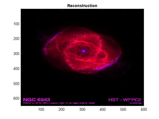
Reconstruct the image using the red and blue components of the coefficients. Display the reconstruction.

llx = ll;
llx(:,:,2) = 0;
for k=1:lvl
    lhx{k} = lh{k};
    hlx{k} = hl{k};
    hhx{k} = hh{k};
    lhx{k}(:,:,2) = 0;
    hlx{k}(:,:,2) = 0;
    hhx{k}(:,:,2) = 0;
end
xrec = ilwt2(llx,lhx,hlx,hhx,LiftingScheme=lScheme,Int2Int=true);
imagesc(uint8(xrec))
title("Reconstruction")

Figure contains an axes object. The axes object with title Reconstruction contains an object of type image.

Confirm the reconstruction is integer valued.

recDiffs = xrec-floor(xrec);
max(abs(recDiffs(:)))

ans = 
0

Input Arguments

collapse all

`x` — Input data
matrix

Input data, specified as a real- or complex-valued 2-D, 3-D, or 4-D matrix. The input x must have at least two samples in the row and column dimensions.

If size(x,1) is odd, the function extends x by duplicating the last row.
If size(x,2) is odd, the function extends the last column of x by duplicating the last column.

Data Types: single | double
Complex Number Support: Yes

Name-Value Arguments

Specify optional pairs of arguments as Name1=Value1,...,NameN=ValueN, where Name is the argument name and Value is the corresponding value. Name-value arguments must appear after other arguments, but the order of the pairs does not matter.

Example: [ll,lh,hl,hh] = lwt2(x,LiftingScheme=lscheme,Level=2)

`Wavelet` — Wavelet
`"db1"` (default) | character vector | string scalar

Orthogonal or biorthogonal wavelet to use in the 2-D LWT, specified as a character vector or string scalar. See the Wavelet property of liftingScheme for the list of supported wavelets.

You cannot specify Wavelet and LiftingScheme at the same time.

Example: [ll,~,~,hh] = lwt2(x,Wavelet="bior3.5") uses the bior3.5 biorthogonal wavelet.

Data Types: char | string

`LiftingScheme` — Lifting scheme
`liftingScheme` object

Lifting scheme to use in the 2-D LWT, specified as a liftingScheme object.

You cannot specify LiftingScheme and Wavelet at the same time.

Example: [~,lh,hl,~] = lwt2(x,LiftingScheme=lScheme) uses the lScheme lifting scheme.

`Level` — Decomposition level
positive integer

Decomposition level of the 2-D LWT, specified as a positive integer less than or equal to floor(log2(N)), where N = min(size(x,[1 2])/2).

The default decomposition level depends on the number of rows and columns in x.

If the number of both the rows and the columns is a power of two, the function performs 2-D LWT down to level log2(min(size(x,[1 2]))).
If the number of both the rows and the columns is even but at least one is not a power of two, the function performs 2-D LWT down to floor(log2(N)), where N = min(size(x,[1 2])/2).

Example: [ll,~,hl,~] = lwt2(x,Level=4) specifies a level 4 wavelet decomposition.

Data Types: double

`Extension` — Extension mode
`"periodic"` (default) | `"zeropad"` | `"symmetric"`

Extension mode to use in the LWT, specified as one of these:

"periodic" — Periodized extension
"zeropad" — Zero extension
"symmetric" — Symmetric extension

This argument specifies how lwt2 extends the input at the boundaries.

Example: [~,lh,~,hh] = lwt2(x,Extension="symmetric") specifies the symmetric extension mode.

Data Types: char | string

`Int2Int` — Handling integer-valued data
`false` or `0` (default) | `true` or `1`

Handling integer-valued data, specified as one of these:

1 (true) — Preserve integer-valued data
0 (false) — Do not preserve integer-valued data

Specify Int2Int only if all elements of the input are integers.

Example: [~,lh,hl,hh] = lwt2(x,Int2Int=true) preserves integer-valued data.

Output Arguments

collapse all

`ll` — Approximation coefficients
scalar | vector | matrix

Approximation coefficients at the coarsest scale, returned as a scalar, vector, or matrix.

Data Types: single | double

`lh` — Horizontal detail coefficients
cell array

Horizontal detail coefficients by level, returned as a LEV-by-1 cell array, where LEV is the level of the decomposition. The elements of lh are in order of decreasing resolution.

Data Types: single | double

`hl` — Vertical detail coefficients
cell array

Vertical detail coefficients by level, returned as a LEV-by-1 cell array, where LEV is the level of the decomposition. The elements of hl are in order of decreasing resolution.

Data Types: single | double

`hh` — Diagonal detail coefficients
cell array

Diagonal detail coefficients by level, returned as a LEV-by-1 cell array, where LEV is the level of the decomposition. The elements of hh are in order of decreasing resolution.

Data Types: single | double

Algorithms

At each stage of a 2-D wavelet decomposition, the approximation coefficients at level j are decomposed into four components: the approximation at level j+1 and the details in three orientations (horizontal, vertical, and diagonal). Each component is the result of convolving the rows and columns of the level j approximation with the appropriate combination of lowpass and highpass filters, LoD and HiD, respectively, followed by downsampling:

Approximation — Convolve the rows and columns with a lowpass filter (ll)
Horizontal — Convolve the rows with a lowpass filter, and convolve the columns with a highpass filter (lh)
Vertical — Convolve the rows with a highpass filter, and convolve the columns with a lowpass filter (hl)
Diagonal — Convolve the rows and columns with a highpass filter (hh)

The following chart describes the basic decomposition steps.

where

— Downsample columns: keep the even-indexed columns
— Downsample rows: keep the even-indexed rows
— Convolve the rows of the entry with filter X
— Convolve the columns of the entry with filter X

The decomposition is initialized by setting the approximation coefficients equal to the image s: cA₀ = s.

References

[1] Daubechies, Ingrid. Ten Lectures on Wavelets. CBMS-NSF Regional Conference Series in Applied Mathematics 61. Philadelphia, Pa: Society for Industrial and Applied Mathematics, 1992.

[2] Mallat, S.G. “A Theory for Multiresolution Signal Decomposition: The Wavelet Representation.” IEEE Transactions on Pattern Analysis and Machine Intelligence 11, no. 7 (July 1989): 674–93. https://doi.org/10.1109/34.192463.

[3] Strang, Gilbert, and Truong Nguyen. Wavelets and Filter Banks. Rev. ed. Wellesley, Mass: Wellesley-Cambridge Press, 1997.

[4] Sweldens, Wim. “The Lifting Scheme: A Construction of Second Generation Wavelets.” SIAM Journal on Mathematical Analysis 29, no. 2 (March 1998): 511–46. https://doi.org/10.1137/S0036141095289051.

Extended Capabilities

C/C++ Code Generation
Generate C and C++ code using MATLAB® Coder™.

Version History

Introduced in R2021b

expand all

R2021b: `lwt2` input syntax has changed

The lwt2 input syntax has changed. Use name-value arguments instead.

Functionality	Result	Use Instead	Compatibility Considerations
`[CA,CH,CV,CD] = lwt2(X,W)`	Errors	`[CA,CH,CV,CD] = lwt2(X,Wavelet=W)`	You can also obtain the lifting wavelet transform (LWT) using a lifting scheme by setting the `LiftingScheme` name-value argument.
`[CA,CH,CV,CD] = lwt2(X,W,LEVEL)`	Errors	`[CA,CH,CV,CD] = lwt2(X,Wavelet=W,Level=LEVEL)`	You can also specify the extension mode by setting the `Extension` name-value argument.
`[CA,CD] = lwt2(X,W,LEVEL,'typeDEC','wp')`	Errors	NA	The wavelet packet decomposition option is no longer provided.
`X_InPlace = lwt2(X,LS)`	Errors	NA	In-place transforms are no longer supported.

lwt2

Syntax

Description

Examples

Lifting Wavelet Transform of 2-D Data

Lifting Wavelet Transform of RGB Image Using Lifting Scheme

Input Arguments

x — Input data matrix

Name-Value Arguments

Wavelet — Wavelet "db1" (default) | character vector | string scalar

LiftingScheme — Lifting scheme liftingScheme object

Level — Decomposition level positive integer

Extension — Extension mode "periodic" (default) | "zeropad" | "symmetric"

Int2Int — Handling integer-valued data false or 0 (default) | true or 1

Output Arguments

ll — Approximation coefficients scalar | vector | matrix

lh — Horizontal detail coefficients cell array

hl — Vertical detail coefficients cell array

hh — Diagonal detail coefficients cell array

Algorithms

References

Extended Capabilities

C/C++ Code Generation Generate C and C++ code using MATLAB® Coder™.

Version History

R2021b: lwt2 input syntax has changed

See Also

`x` — Input data
matrix

`Wavelet` — Wavelet
`"db1"` (default) | character vector | string scalar

`LiftingScheme` — Lifting scheme
`liftingScheme` object

`Level` — Decomposition level
positive integer

`Extension` — Extension mode
`"periodic"` (default) | `"zeropad"` | `"symmetric"`

`Int2Int` — Handling integer-valued data
`false` or `0` (default) | `true` or `1`

`ll` — Approximation coefficients
scalar | vector | matrix

`lh` — Horizontal detail coefficients
cell array

`hl` — Vertical detail coefficients
cell array

`hh` — Diagonal detail coefficients
cell array

C/C++ Code Generation
Generate C and C++ code using MATLAB® Coder™.

R2021b: `lwt2` input syntax has changed