mlptrecon
Reconstruct signal using inverse multiscale local 1-D polynomial transform
Description
Examples
Create a low-frequency signal with high-frequency blips.
t = (0:0.01:10)';
x = sin(2*pi.*t) + 0.5*sin(pi.*t+0.1);
bliptime = (0:0.01:0.5)';
n = numel(bliptime);
z0 = 2*(1:(n+1)/2)/(n+1);
trng = [z0 z0((n-1)/2:-1:1)]';
blip = sin(50*pi.*bliptime).*trng;
for i = [200,700,900]
    x(i:i+numel(bliptime)-1) = x(i:i+numel(bliptime)-1)+blip;
end
Perform a multilevel polynomial transform. Perform the inverse multilevel polynomial transform using the detail coefficients.
[w,t,nj,scalingmoments] = mlpt(x,t);
yDetails = mlptrecon('d',w,t,nj,scalingmoments,1);
Plot the original signal and the processed signal.
subplot(2,1,1)
plot(t,x)
title('Original Signal')

subplot(2,1,2)
plot(t,yDetails)
title('Signal Details')

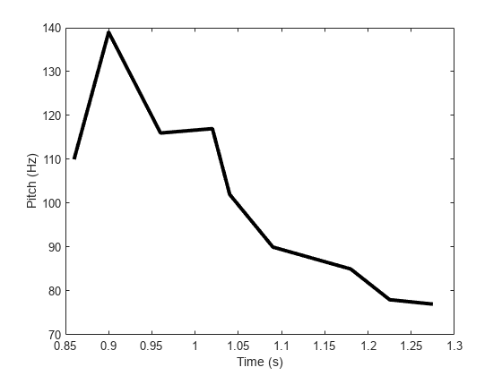
Approximate data using multiscale local polynomial transform (MLPT) reconstruction. Use mlptrecon to approximate a corrupted and sparsely sampled pitch contour.
Load input data and visualize it.
load CorruptedPitchData.mat
plot(time,pitchContour,'k',linewidth=3)
hold on
xlabel('Time (s)')
ylabel('Pitch (Hz)')
Compute the MLPT of the pitch contour.
[w,t,nj,scalingMoments] = mlpt(pitchContour,time, ...
    DualMoments=3, ...
    PrimalMoments=4, ...
    PreFilter='none');
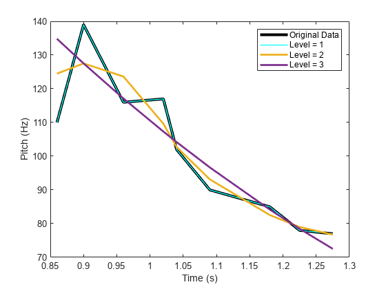
Use mlptrecon to reconstruct the signal using the approximation coefficients at different levels.
y = zeros(numel(t),3);
for level = 1:3
    y(:,level) = mlptrecon('a',w,t,nj,scalingMoments,level, ...
        DualMoments=3);
end
Plot the reconstructed signals. Level two obtains the best smoothed estimate.
plot(t,y(:,1),'c',linewidth=1)
plot(t,y(:,2),linewidth=2)
plot(t,y(:,3),linewidth=2)
legend('Original Data','Level = 1','Level = 2','Level = 3')
hold off
Input Arguments
Output Arguments
Algorithms
Maarten Jansen developed the theoretical foundation of the multiscale
local polynomial transform (MLPT) and algorithms for its efficient
computation [1][2][3]. The MLPT uses a lifting scheme, wherein a kernel
function smooths fine-scale coefficients with a given bandwidth to
obtain the coarser resolution coefficients. The mlpt function uses only local polynomial
interpolation, but the technique developed by Jansen is more general
and admits many other kernel types with adjustable bandwidths [2].
References
[1] Jansen, Maarten. “Multiscale Local Polynomial Smoothing in a Lifted Pyramid for Non-Equispaced Data.” IEEE Transactions on Signal Processing 61, no. 3 (February 2013): 545–55. https://doi.org/10.1109/TSP.2012.2225059.
[2] Jansen, Maarten, and Mohamed Amghar. “Multiscale Local Polynomial Decompositions Using Bandwidths as Scales.” Statistics and Computing 27, no. 5 (September 2017): 1383–99. https://doi.org/10.1007/s11222-016-9692-8.
[3] Jansen, Maarten, and Patrick Oonincx. Second Generation Wavelets and Applications. London ; New York: Springer, 2005.
Version History
Introduced in R2017a