swt2

Discrete stationary 2-D wavelet transform

Syntax

[A,H,V,D] = swt2(X,N,wname)

[A,H,V,D] = swt2(X,N,LoD,HiD)

swc = swt2(___)

Description

[A,H,V,D] = swt2(X,N,wname) returns the approximation coefficients A and the horizontal, vertical, and diagonal detail coefficients H, V, and D, respectively, of the stationary 2-D wavelet decomposition of the image X at level N using the wavelet wname.

Note

swt2 is uses periodic extension.
swt2 uses double-precision arithmetic internally and returns double-precision coefficient matrices. swt2 warns if there is a loss of precision when converting to double.

example

[A,H,V,D] = swt2(X,N,LoD,HiD) uses the specified lowpass and highpass wavelet decomposition filters LoD and HiD, respectively.

swc = swt2(___) returns the approximation and detail coefficients in swc.

Examples

collapse all

Extract and Display 2-D Stationary Wavelet Decomposition

Open Live Script

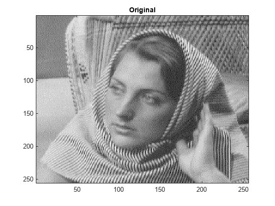
Load and display an image.

load woman
imagesc(X)
colormap(map)
title('Original')

Figure contains an axes object. The axes object with title Original contains an object of type image.

Perform the stationary wavelet decomposition of the image at level 2 using db6.

[ca,chd,cvd,cdd] = swt2(X,2,'db6');

Extract the level 1 and level 2 approximation and detail coefficients from the decomposition.

A1 = wcodemat(ca(:,:,1),255);
H1 = wcodemat(chd(:,:,1),255);
V1 = wcodemat(cvd(:,:,1),255);
D1 = wcodemat(cdd(:,:,1),255);

A2 = wcodemat(ca(:,:,2),255);
H2 = wcodemat(chd(:,:,2),255);
V2 = wcodemat(cvd(:,:,2),255);
D2 = wcodemat(cdd(:,:,2),255);

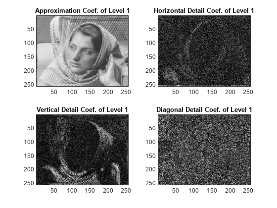
Display the approximation and detail coefficients from the two levels.

subplot(2,2,1)
imagesc(A1)
title('Approximation Coef. of Level 1')

subplot(2,2,2)
imagesc(H1)
title('Horizontal Detail Coef. of Level 1')

subplot(2,2,3)
imagesc(V1)
title('Vertical Detail Coef. of Level 1')

subplot(2,2,4)
imagesc(D1)
title('Diagonal Detail Coef. of Level 1')

Figure contains 4 axes objects. Axes object 1 with title Approximation Coef. of Level 1 contains an object of type image. Axes object 2 with title Horizontal Detail Coef. of Level 1 contains an object of type image. Axes object 3 with title Vertical Detail Coef. of Level 1 contains an object of type image. Axes object 4 with title Diagonal Detail Coef. of Level 1 contains an object of type image.

subplot(2,2,1)
imagesc(A2)
title('Approximation Coef. of Level 2')

subplot(2,2,2)
imagesc(H2)
title('Horizontal Detail Coef. of Level 2')

subplot(2,2,3)
imagesc(V2)
title('Vertical Detail Coef. of Level 2')

subplot(2,2,4)
imagesc(D2)
title('Diagonal Detail Coef. of Level 2')

Figure contains 4 axes objects. Axes object 1 with title Approximation Coef. of Level 2 contains an object of type image. Axes object 2 with title Horizontal Detail Coef. of Level 2 contains an object of type image. Axes object 3 with title Vertical Detail Coef. of Level 2 contains an object of type image. Axes object 4 with title Diagonal Detail Coef. of Level 2 contains an object of type image.

Stationary Wavelet Transform of RGB Image

Open Live Script

This example shows how to obtain single-level and multilevel stationary wavelet decompositions of an RGB image.

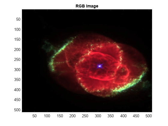
Load and view an RGB image. The image is a 3-D array of type uint8. Since swt2 requires that the first and second dimensions both be divisible by a power of 2, extract a portion of the image.

imdata = imread('ngc6543a.jpg');
x = imdata(1:512,1:512,:);
image(x)
title('RGB Image')

Figure contains an axes object. The axes object with title RGB Image contains an object of type image.

Obtain the level 4 stationary wavelet decomposition of the image using the db4 wavelet. Return the approximation coefficients. Note the dimensions of the coefficients array.

[a,~,~,~] = swt2(x,4,'db4');
size(a)

ans = 1×4

   512   512     3     4

The coefficients are all of type double. In an RGB array of type double, each color component is a value between 0 and 1. Rescale the level 2 approximation coefficients to values between 0 and 1 and view the result.

a2 = a(:,:,:,2);
a2 = (a2-min(a2(:)))/(max(a2(:))-min(a2(:)));
image(a2)
title('Level 2 Approximation')

Figure contains an axes object. The axes object with title Level 2 Approximation contains an object of type image.

Obtain the single-level stationary wavelet decomposition of the image using the db4 wavelet. Return the approximation coefficients. In a single-level decomposition of an RGB image, the third dimension is singleton.

[a,~,~,~] = swt2(x,1,'db4');
size(a)

ans = 1×4

   512   512     1     3

View the approximation coefficients. To prevent an error when using image, squeeze the approximation coefficients array to remove the singleton dimension.

a2 = squeeze(a);
a2 = (a2-min(a(:)))/(max(a(:))-min(a(:)));
image(a2)
title('Approximation')

Figure contains an axes object. The axes object with title Approximation contains an object of type image.

Input Arguments

collapse all

`X` — Input image
2-D matrix | 3-D array

Input image, specified as a real-valued 2-D matrix or real-valued 3-D array. If X is 3-D, X is assumed to be an RGB image, also referred to as a truecolor image, and the third dimension of X must equal 3. For more information on truecolor images, see Working with Image Types in MATLAB.

Data Types: double

`N` — Level of decomposition
positive integer

Level of decomposition, specified as a positive integer. 2^N must divide size(X,1) and size(X,2). Use wmaxlev to determine the maximum level of decomposition.

`wname` — Analyzing wavelet
character vector | string scalar

Analyzing wavelet, specified as a character vector or string scalar. swt2 supports only Type 1 (orthogonal) or Type 2 (biorthogonal) wavelets. See wfilters for a list of orthogonal and biorthogonal wavelets.

`LoD,HiD` — Wavelet decomposition filters
even-length real-valued vectors

Wavelet decomposition filters, specified as a pair of even-length real-valued vectors. LoD is the lowpass decomposition filter, and HiD is the highpass decomposition filter. The lengths of LoD and HiD must be equal. See wfilters for additional information.

Output Arguments

collapse all

`A` — Approximation coefficients
2-D matrix | 3-D array | 4-D array

Approximation coefficients, returned as a multidimensional array. The dimensions of A depend on the dimensions of the input X and the level of decomposition N.

If X is m-by-n:
- If N is greater than 1, then A is m-by-n-by-N. For 1 ≤ i ≤ N, A(:,:,i) contains the approximation coefficients at level i.
- If N is equal to 1, then A is m-by-n.
If X is m-by-n-by-3:
- If N is greater than 1, then A is m-by-n-by-3-by-N. For 1 ≤ i ≤ N and j = 1, 2, 3, A(:,:,j,i) contains approximation coefficients at level i.
- If N is equal to 1, then A is m-by-n-by-1-by-3. Since MATLAB^® removes singleton last dimensions by default, the third dimension is singleton.

Data Types: double

`H,V,D` — Detail coefficients
2-D matrix | 3-D array | 4-D array

Detail coefficients, returned as multidimensional arrays of equal size. H, V, and D contain the horizontal, vertical, and diagonal detail coefficients, respectively. The dimensions of the arrays depend on the dimensions of the input X and the level of decomposition N.

If X is m-by-n:
- If N is greater than 1, the arrays are m-by-n-by-N. For 1 ≤ i ≤ N, H(:,:,i), V(:,:,i), and D(:,:,i) contain the detail coefficients at level i.
- If N is equal to 1, the arrays are m-by-n.
If X is m-by-n-by-3:
- If N is greater than 1, the arrays are m-by-n-by-3-by-N. For 1 ≤ i ≤ N and j = 1, 2, 3, H(:,:,j,i), V(:,:,j,i), and D(:,:,j,i) contain the detail coefficients at level i.
- If N is equal to 1, the arrays are m-by-n-by-1-by-3. For j = 1, 2, 3, H(:,:,1,j), V(:,:,1,j) and D(:,:,1,j) contain the detail coefficients. Since MATLAB removes singleton last dimensions by default, the third dimension is singleton.

Data Types: double

`swc` — Stationary wavelet decomposition
3-D array | 4-D array

Stationary wavelet decomposition, returned as a multidimensional array. swc is the concatenation of the approximation coefficients A and detail coefficients H, V, and D.

If X is m-by-n and N is greater than 1, then swc = cat(3,H,V,D,A(:,:,N)).
If X is m-by-n and N is equal to 1, then swc = cat(3,H,V,D,A).
If X is m-by-n-by-3 and N is greater than 1, then swc = cat(4,H,V,D,A(:,:,:,N)).
If X is m-by-n-by-3 and N is equal to1, then swc = cat(4,H,V,D,A).

Algorithms

collapse all

2-D Discrete Stationary Wavelet Transform

For images, a stationary wavelet transform (SWT) algorithm similar to the one-dimensional case is possible for two-dimensional wavelets and scaling functions obtained from one-dimensional functions by tensor product. This kind of two-dimensional SWT leads to a decomposition of approximation coefficients at level j into four components: the approximation at level j+1, and the details in three orientations (horizontal, vertical, and diagonal).

This chart describes the basic decomposition step for images.

where

— Convolve the rows of the entry with filter X.
— Convolve the columns of the entry with filter X.

Initialization

cA₀ = s
F₀ = LoD
G₀ = HiD
where denotes upsample.

Note that size(cA_j) = size(cD_j^(h)) = size(cD_j^(v)) = size(cD_j^(d)) = s, where s equals the size of the analyzed image.

Truecolor Image Coefficient Arrays

To distinguish a single-level decomposition of a truecolor image from a multilevel decomposition of an indexed image, the approximation and detail coefficient arrays of truecolor images are 4-D arrays.

If you perform a multilevel decomposition, the dimensions of A, H, V, and D are m-by-n-by-3-by-k, where k is the level of decomposition.
If you perform a single-level decomposition, the dimensions of A, H, V, and D are m-by-n-by-1-by-3. Since MATLAB removes singleton last dimensions by default, the third dimension of the arrays is singleton.

References

[1] Nason, G. P., and B. W. Silverman. “The Stationary Wavelet Transform and Some Statistical Applications.” In Wavelets and Statistics, edited by Anestis Antoniadis and Georges Oppenheim, 103:281–99. New York, NY: Springer New York, 1995. https://doi.org/10.1007/978-1-4612-2544-7_17.

[2] Coifman, R. R., and D. L. Donoho. “Translation-Invariant De-Noising.” In Wavelets and Statistics, edited by Anestis Antoniadis and Georges Oppenheim, 103:125–50. New York, NY: Springer New York, 1995. https://doi.org/10.1007/978-1-4612-2544-7_9.

[3] Pesquet, J.-C., H. Krim, and H. Carfantan. “Time-Invariant Orthonormal Wavelet Representations.” IEEE Transactions on Signal Processing 44, no. 8 (August 1996): 1964–70. https://doi.org/10.1109/78.533717.

Extended Capabilities

C/C++ Code Generation
Generate C and C++ code using MATLAB® Coder™.

Usage notes and limitations:

The input wavelet name must be constant.
The input level of decomposition must be defined as a scalar during compilation.

Version History

Introduced before R2006a

expand all

R2017b: Distinguish Single-Level Truecolor Image from Multilevel Indexed Image Decompositions

To distinguish a single-level decomposition of a truecolor image from a multilevel decomposition of an indexed image, the approximation and detail coefficient arrays of truecolor images are 4-D arrays.

Migrate from Previous Releases to R2017b

Depending on the original input data type and level of wavelet decomposition, you might have to take different steps to make swt2 coefficient arrays from previous releases compatible with R2017b coefficient arrays. The steps depend on whether you have a single coefficient array or separate approximation and detail coefficient arrays.

Single Coefficient Array Multiple Coefficient Arrays

Single Coefficient Array	Multiple Coefficient Arrays
Input: Index image Single-level: No compatibility issues Multi-level: No compatibility issues	Input: Index image Single-level: No compatibility issues Multi-level: No compatibility issues
Input: Truecolor image Single-level: If `swc` is the output of `swt2` from a previous release, execute: swc1 = double(swc); Multi-level: If `swc` is the output of `swt2` from a previous release, execute: swc1 = double(swc);	Input: Truecolor image Single-level: If `ca`, `chd`, `cvd`, and `cdd` are outputs of `swt2` from a previous release, execute: ca1 = double(ca); chd1 = double(chd); cvd1 = double(cvd); cdd1 = double(cdd); ca2 = reshape(ca1,[m,n,1,3]); chd2 = reshape(chd1,[m,n,1,3]); cvd2 = reshape(cvd1,[m,n,1,3]); cdd2 = reshape(cdd1,[m,n,1,3]); Multi-level: If `ca`, `chd`, `cvd`, and `cdd` are outputs of `swt2` from a previous release, execute: ca1 = double(ca); chd1 = double(chd); cvd1 = double(cvd); cdd1 = double(cdd);

Input: Index image

Single-level: No compatibility issues
Multi-level: No compatibility issues

Input: Index image

Single-level: No compatibility issues
Multi-level: No compatibility issues

Input: Truecolor image

Single-level: If swc is the output of swt2 from a previous release, execute:
```
swc1 = double(swc);
```
Multi-level: If swc is the output of swt2 from a previous release, execute:
```
swc1 = double(swc);
```

Input: Truecolor image

Single-level: If ca, chd, cvd, and cdd are outputs of swt2 from a previous release, execute:

ca1 = double(ca);
chd1 = double(chd);
cvd1 = double(cvd);
cdd1 = double(cdd);
ca2 = reshape(ca1,[m,n,1,3]);
chd2 = reshape(chd1,[m,n,1,3]);
cvd2 = reshape(cvd1,[m,n,1,3]);
cdd2 = reshape(cdd1,[m,n,1,3]);

Multi-level: If ca, chd, cvd, and cdd are outputs of swt2 from a previous release, execute:
```
ca1 = double(ca);
chd1 = double(chd);
cvd1 = double(cvd);
cdd1 = double(cdd);
```

Migrate from R2017b to Previous Releases

Depending on the original input data type and level of wavelet decomposition, you might have to take different steps to make R2017b swt2 coefficient arrays compatible with the coefficient arrays from previous releases. The steps depend on whether you have a single coefficient array or separate approximation and detail coefficient arrays.

Single Coefficient Array Multiple Coefficient Arrays

Single Coefficient Array	Multiple Coefficient Arrays
Input: Index image Single-level: No compatibility issues Multi-level: No compatibility issues	Input: Index image Single-level: No compatibility issues Multi-level: No compatibility issues
Input: Truecolor image Single-level: No compatibility issues Multi-level: No compatibility issues	Input: Truecolor image Single-level: If `ca`, `chd`, `cvd`, and `cdd` are outputs of `swt2` from R2017b, execute: ca1 = single(squeeze(ca)); chd1 = single(squeeze(chd)); cvd1 = single(squeeze(cvd)); cdd1 = single(squeeze(cdd)); Multi-level: No compatibility issues

Input: Index image

Single-level: No compatibility issues
Multi-level: No compatibility issues

Input: Index image

Single-level: No compatibility issues
Multi-level: No compatibility issues

Input: Truecolor image

Single-level: No compatibility issues
Multi-level: No compatibility issues

Input: Truecolor image

Single-level: If ca, chd, cvd, and cdd are outputs of swt2 from R2017b, execute:

ca1 = single(squeeze(ca));
chd1 = single(squeeze(chd));
cvd1 = single(squeeze(cvd));
cdd1 = single(squeeze(cdd));

Multi-level: No compatibility issues

swt2

Syntax

Description

Examples

Extract and Display 2-D Stationary Wavelet Decomposition

Stationary Wavelet Transform of RGB Image

Input Arguments

X — Input image 2-D matrix | 3-D array

N — Level of decomposition positive integer

wname — Analyzing wavelet character vector | string scalar

LoD,HiD — Wavelet decomposition filters even-length real-valued vectors

Output Arguments

A — Approximation coefficients 2-D matrix | 3-D array | 4-D array

H,V,D — Detail coefficients 2-D matrix | 3-D array | 4-D array

swc — Stationary wavelet decomposition 3-D array | 4-D array

Algorithms

2-D Discrete Stationary Wavelet Transform

Truecolor Image Coefficient Arrays

References

Extended Capabilities

C/C++ Code Generation Generate C and C++ code using MATLAB® Coder™.

Version History

R2017b: Distinguish Single-Level Truecolor Image from Multilevel Indexed Image Decompositions

See Also

`X` — Input image
2-D matrix | 3-D array

`N` — Level of decomposition
positive integer

`wname` — Analyzing wavelet
character vector | string scalar

`LoD,HiD` — Wavelet decomposition filters
even-length real-valued vectors

`A` — Approximation coefficients
2-D matrix | 3-D array | 4-D array

`H,V,D` — Detail coefficients
2-D matrix | 3-D array | 4-D array

`swc` — Stationary wavelet decomposition
3-D array | 4-D array

C/C++ Code Generation
Generate C and C++ code using MATLAB® Coder™.