Main Content

wavefun

Wavelet and scaling functions

Description

[phi,psi,xval] = wavefun(wname,iter) returns psi and phi, approximations of the wavelet and scaling functions, respectively, associated with the orthogonal wavelet wname, or the Meyer wavelet. The approximations are evaluated on the grid points xval. The positive integer iter specifies the number of iterations computed.

example

[phi1,psi1,phi2,psi2,xval] = wavefun(wname,iter) returns approximations of the wavelet and scaling functions associated with the biorthogonal wavelet wname. The wavelet and scaling function approximations psi1 and phi1, respectively, are for decomposition. The wavelet and scaling function approximations psi2 and phi2, respectively, are for reconstruction.

[psi,xval] = wavefun(wname,iter) returns the wavelet approximation psi for those wavelets that do not have an associated scaling function, such as Morlet, Mexican Hat, Gaussian derivatives wavelets, or complex wavelets.

[___] = wavefun(___,"plot") also plots the functions.

[___] = wavefun(wname,A,B) returns and plots the wavelet and scaling function approximations generated using max(A,B) iterations.

  • wavefun(wname,0) is equivalent to wavefun(wname,8,0).

  • wavefun(wname) is equivalent to wavefun(wname,8).

example

Examples

collapse all

This example shows how the number of iterations affects the piecewise approximation of the specified wavelet.

Specify the number of iterations and the wavelet name.

wname = "sym4";
itr = 10;

Plot the piecewise approximation of the wavelet generated after one iteration.

[~,psi,xval] = wavefun(wname,1);
plot(xval,psi,'x-')
grid on
title("Approximation of "+wname+" Wavelet")

Figure contains an axes object. The axes object with title Approximation of sym4 Wavelet contains an object of type line.

Vary the number of iterations from 1 to 4 and plot the approximations. Observe that as the number of iterations grows, so do the number of sample points.

tiledlayout(2,2)
for k=1:4
    [~,psi,xval] = wavefun(wname,k);
    nexttile
    plot(xval,psi,'x-')
    axis tight
    grid on
    title("Number of Iterations: "+num2str(k))
end

Figure contains 4 axes objects. Axes object 1 with title Number of Iterations: 1 contains an object of type line. Axes object 2 with title Number of Iterations: 2 contains an object of type line. Axes object 3 with title Number of Iterations: 3 contains an object of type line. Axes object 4 with title Number of Iterations: 4 contains an object of type line.

Now vary the number of iterations from 1 to 10. Plot the approximations for all iterations.

figure
for k=1:10
    [~,psi,xval] = wavefun(wname,k);
    plot(xval,psi)
    hold on
end
hold off
grid on
title("Ten Approximations of "+wname+" Wavelet")

Figure contains an axes object. The axes object with title Ten Approximations of sym4 Wavelet contains 10 objects of type line.

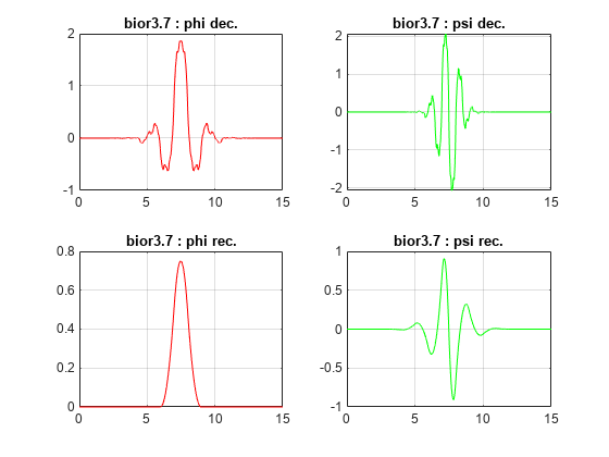
This example shows how to plot approximations of the scaling and wavelet functions associated with a biorthogonal wavelet.

Specify the name of a biorthogonal wavelet.

wname = "bior3.7";

Plot approximations of the scaling and wavelet functions associated with the specified biorthogonal wavelet using the default number of iterations. Plot the approximations for both decomposition and reconstruction.

wavefun(wname,0);

Figure contains 4 axes objects. Axes object 1 with title bior3.7 : phi dec. contains an object of type line. Axes object 2 with title bior3.7 : psi dec. contains an object of type line. Axes object 3 with title bior3.7 : phi rec. contains an object of type line. Axes object 4 with title bior3.7 : psi rec. contains an object of type line.

Input Arguments

collapse all

Wavelet, specified as a character vector or string scalar. See waveinfo for wavelets available.

Number of iterations used to generate the wavelet and scaling function approximations, specified as a positive integer. Larger values of iter increase the refinement of the approximations.

Iteration, specified as a pair of positive integers. The number of iterations is equal to max(A,B).

Output Arguments

collapse all

Scaling function approximation, returned as a vector.

Wavelet approximation, returned as a vector. Depending on wname, psi can be a real- or complex-valued vector.

Approximations of decomposition scaling and wavelet functions, respectively, associated with the biorthogonal wavelet wname, returned as real-valued vectors.

Approximations of reconstruction scaling and wavelet functions, respectively, associated with the biorthogonal wavelet wname, returned as real-valued vectors.

Grid points where the wavelet and scaling function approximations are evaluated, returned as a real-valued vector.

Algorithms

For compactly supported wavelets defined by filters, in general no closed form analytic formula exists.

The algorithm used is the cascade algorithm. It uses the single-level inverse wavelet transform repeatedly.

Let us begin with the scaling function ϕ.

Since ϕ is also equal to ϕ0,0, this function is characterized by the following coefficients in the orthogonal framework:

  • <ϕ, ϕ0,n> = 1 only if n = 0 and equal to 0 otherwise

  • <ϕ, ψ−j,k> = 0 for positive j, and all k.

This expansion can be viewed as a wavelet decomposition structure. Detail coefficients are all zeros and approximation coefficients are all zeros except one equal to 1.

Then we use the reconstruction algorithm to approximate the function ϕ over a dyadic grid, according to the following result:

For any dyadic rational of the form x = n2−j in which the function is continuous and where j is sufficiently large, we have pointwise convergence and

where C is a constant, and α is a positive constant depending on the wavelet regularity.

Then using a good approximation of ϕ on dyadic rationals, we can use piecewise constant or piecewise linear interpolations η on dyadic intervals, for which uniform convergence occurs with similar exponential rate:

So using a J-step reconstruction scheme, we obtain an approximation that converges exponentially towards ϕ when J goes to infinity.

Approximations are computed over a grid of dyadic rationals covering the support of the function to be approximated.

Since a scaled version of the wavelet function ψ can also be expanded on the (ϕ−1,n))n, the same scheme can be used, after a single-level reconstruction starting with the appropriate wavelet decomposition structure. Approximation coefficients are all zeros and detail coefficients are all zeros except one equal to 1.

For biorthogonal wavelets, the same ideas can be applied on each of the two multiresolution schemes in duality.

Note

This algorithm may diverge if the function to be approximated is not continuous on dyadic rationals.

References

[1] Daubechies, I. Ten Lectures on Wavelets. CBMS-NSF Regional Conference Series in Applied Mathematics. Philadelphia, PA: Society for Industrial and Applied Mathematics, 1992.

[2] Strang, G., and T. Nguyen. Wavelets and Filter Banks. Wellesley, MA: Wellesley-Cambridge Press, 1996.

Version History

Introduced before R2006a