wden

This example shows how to apply three different denoising techniques to a noisy signal. It compares the results with plots and the threshold values produced by each technique.

First, to ensure reproducibility of results, set a seed that will be used to generate the random noise.

rng('default')

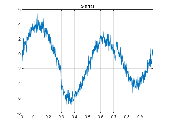
Create a signal consisting of a 2 Hz sine wave with transients at 0.3 and 0.72 seconds. Add randomly generated noise to the signal and plot the result.

N = 1000;
t = linspace(0,1,N);
x = 4*sin(4*pi*t);
x = x - sign(t-0.3) - sign(0.72-t);
sig = x + 0.5*randn(size(t));
plot(t,sig)
title('Signal')
grid on

Using the sym8 wavelet, perform a level 5 wavelet decomposition of the signal and denoise it by applying three different threshold selection rules to the wavelet coefficients: SURE, minimax, and Donoho and Johnstone's universal threshold with level-dependent estimation of the noise. In each case, apply hard thresholding.

lev = 5;
wname = 'sym8';
[dnsig1,c1,l1,threshold_SURE] = wden(sig,'rigrsure','h','mln', ...
    lev,wname);
[dnsig2,c2,l2,threshold_Minimax] = wden(sig,'minimaxi','h','mln', ...
    lev,wname);
[dnsig3,c3,l3,threshold_DJ] = wden(sig,'sqtwolog','h','mln', ...
    lev,wname);

Plot and compare the three denoised signals.

tiledlayout(3,1)
nexttile
plot(t,dnsig1)
title('Denoised Signal - SURE')
grid on
nexttile
plot(t,dnsig2)
title('Denoised Signal - Minimax')
grid on
nexttile
plot(t,dnsig3)
title('Denoised Signal - Donoho-Johnstone')
grid on

Compare the thresholds applied at each detail level for the three denoising methods.

threshold_SURE

threshold_SURE = 1×5

    0.9592    0.6114    1.4734    0.7628    0.4360

threshold_Minimax

threshold_Minimax = 1×5

    1.1047    1.0375    1.3229    1.1245    1.0483

threshold_DJ

threshold_DJ = 1×5

    1.8466    1.7344    2.2114    1.8798    1.7524

This example denoises a signal using the DWT and MODWT. It compares the results with plots and the threshold values produced by each technique.

First, to ensure reproducibility of results, set a seed that will be used to generate random noise.

rng('default')

Create a signal consisting of a 2 Hz sine wave with transients at 0.3 and 0.72 seconds. Add randomly generated noise to the signal and plot the result.

N = 1000;
t = linspace(0,1,N);
x = 4*sin(4*pi*t);
x = x - sign(t-0.3) - sign(0.72-t);
sig = x + 0.5*randn(size(t));
plot(t,sig)
title('Signal')
grid on

Using the db2 wavelet, perform a level 3 wavelet decomposition of the signal and denoise it using Donoho and Johnstone's universal threshold with level-dependent estimation of the noise. Obtain denoised versions using DWT and MODWT, both with soft thresholding.

wname = 'db2';
lev = 3;
[xdDWT,c1,l1,threshold_DWT] = wden(sig,'sqtwolog','s','mln', ...
    lev,wname);
[xdMODWT,c2,threshold_MODWT] = wden(sig,'modwtsqtwolog','s','mln', ...
    lev,wname);

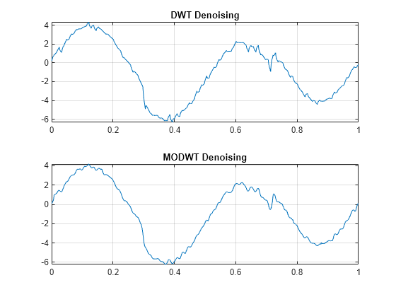
Plot and compare the results.

tiledlayout(2,1)
nexttile
plot(t,xdDWT)
grid on
title('DWT Denoising')
nexttile
plot(t,xdMODWT)
grid on
title('MODWT Denoising')

Compare the thresholds applied in each case.

threshold_DWT

threshold_DWT = 1×3

    1.7783    1.6876    2.0434

threshold_MODWT

threshold_MODWT = 1×3

    1.2760    0.6405    0.3787

This example denoises a blocky signal using the Haar wavelet with DWT and MODWT denoising. It compares the results with plots and metrics for the original and denoised versions.

First, to ensure reproducibility of results, set a seed that will be used to generate random noise.

rng('default')

Generate a signal and a noisy version with the square root of the signal-to-noise ratio equal to 3. Plot and compare each.

[osig,nsig] = wnoise('blocks',10,3);
plot(nsig,'r')
hold on
plot(osig,'b')
legend('Noisy Signal','Original Signal')

Using the Haar wavelet, perform a level 6 wavelet decomposition of the noisy signal and denoise it using Donoho and Johnstone's universal threshold with level-dependent estimation of the noise. Obtain denoised versions using DWT and MODWT, both with soft thresholding.

wname = 'haar';
lev = 6 ;
[xdDWT,c1,l1] = wden(nsig,'sqtwolog','s','mln',lev,wname);
[xdMODWT,c2] = wden(nsig,'modwtsqtwolog','s','mln',lev,wname);

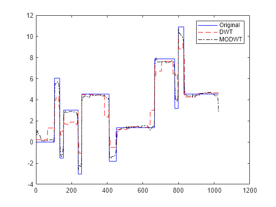
Plot and compare the original, noise-free version of the signal with the two denoised versions.

figure
plot(osig,'b')
hold on
plot(xdDWT,'r--')
plot(xdMODWT,'k-.')
legend('Original','DWT','MODWT')
hold off

Calculate the L2 and L-infinity norms of the difference between the original signal and the two denoised versions.

L2norm_original_DWT = norm(abs(osig-xdDWT),2)

L2norm_original_DWT = 
36.1194

L2norm_original_MODWT = norm(abs(osig-xdMODWT),2)

L2norm_original_MODWT = 
14.5987

LInfinity_original_DWT = norm(abs(osig-xdDWT),Inf)

LInfinity_original_DWT = 
4.7181

LInfinity_original_MODWT = norm(abs(osig-xdMODWT),Inf)

LInfinity_original_MODWT = 
2.9655

References

[1] Antoniadis, A., and G. Oppenheim, eds. Wavelets and Statistics, 103. Lecture Notes in Statistics. New York: Springer Verlag, 1995.
[2] Donoho, D. L. “Progress in Wavelet Analysis and WVD: A Ten Minute Tour.” Progress in Wavelet Analysis and Applications (Y. Meyer, and S. Roques, eds.). Gif-sur-Yvette: Editions Frontières, 1993.
[3] Donoho, D. L., and Johnstone, I. M. “Ideal Spatial Adaptation by Wavelet Shrinkage.” Biometrika, Vol. 81, pp. 425–455, 1994.
[4] Donoho, D. L. “De-noising by Soft-Thresholding.” IEEE Transactions on Information Theory, Vol. 42, Number 3, pp. 613–627, 1995.
[5] Donoho, D. L., I. M. Johnstone, G. Kerkyacharian, and D. Picard. “Wavelet Shrinkage: Asymptopia?” Journal of the Royal Statistical Society, series B. Vol. 57, Number 2, pp. 301–369, 1995.
Extended Capabilities
Version History
Introduced before R2006a