Time-Frequency Reassignment and Mode Extraction with Synchrosqueezing

Open Live Script

This example shows how to use wavelet synchrosqueezing to obtain a higher resolution time-frequency analysis. The example also shows how to extract and reconstruct oscillatory modes in a signal.

In many practical applications across a wide range of disciplines, signals occur which consist of a number of oscillatory components, or modes. These components often exhibit slow variations in amplitude and smooth changes in frequency over time. Signals consisting of one or more such components are called amplitude and frequency modulated (AM-FM). Individual AM-FM components of signals are also referred to as intrinsic modes, or intrinsic mode functions (IMF).

Wavelet synchrosqueezing is a method for analyzing signals consisting of a sum of well-separated AM-FM components, or IMFs. With synchrosqueezing, you can sharpen the time-frequency analysis of a signal as well as reconstruct individual oscillatory modes for isolated analysis.

Sharpen Time-Frequency Analysis

Synchrosqueezing can compensate for the spreading in time and frequency caused by linear transforms like the short-time Fourier and continuous wavelet transforms (CWT). In the CWT, the wavelet acts like a measuring device for the input signal. Accordingly, any time frequency analysis depends not only on the intrinsic time-frequency properties of the signal, but also on the properties of the wavelet.

To demonstrate this, first obtain and plot the CWT of a quadratic chirp signal. The signal's frequency begins at approximately 500 Hz at t = 0, decreases to 100 Hz at t=2, and increases back to 500 Hz at t=4. The sampling frequency is 1 kHz.

load quadchirp
fs = 1000;
[cfs,f] = cwt(quadchirp,"bump",fs);
helperCWTTimeFreqPlot(cfs,tquad,f,"surf","CWT of Quadratic Chirp","Seconds","Hz")

Figure contains an axes object. The axes object with title CWT of Quadratic Chirp, xlabel Seconds, ylabel Hz contains an object of type surface.

Note that the energy of the quadratic chirp is smeared in the time-frequency plane by the time-frequency concentration of the wavelet. For example, if you focus on the time-frequency concentration of the CWT magnitudes near 100 Hz, you see that it is narrower than that observed near 500 Hz. This is not an intrinsic property of the chirp. It is an artifact of the measuring device (the CWT). Compare the time-frequency analysis of the same signal obtained with the synchrosqueezed transform.

wsst(quadchirp,1000,"bump")

Figure contains an axes object. The axes object with title Wavelet Synchrosqueezed Transform, xlabel Time (secs), ylabel Frequency (Hz) contains an object of type surface.

The synchrosqueezed transform uses the phase information in the CWT to sharpen the time-frequency analysis of the chirp.

Reconstruct Signal from Synchrosqueezed Transform

You can reconstruct a signal from the synchrosqueezed transform. This is an advantage synchrosqueezing has over other time-frequency reassignment techniques. The transform does not provide a perfect inversion, but the reconstruction is stable and the results are typically quite good. To demonstrate this, load, plot, and play a recording of a female speaker saying "I saw the sheep".

load wavsheep
plot(tsh,sheep)
title(' "I saw the sheep." ')
xlabel("Time (secs)")
ylabel("Amplitude")
grid on

Figure contains an axes object. The axes object with title "I saw the sheep.", xlabel Time (secs), ylabel Amplitude contains an object of type line.

hplayer = audioplayer(sheep,fs);
play(hplayer)

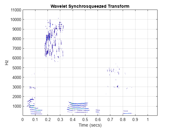
Plot the synchrosqueezed transform of the speech sample.

[sst,f] = wsst(sheep,fs,"bump");
contour(tsh,f,abs(sst))
title("Wavelet Synchrosqueezed Transform")
xlabel("Time (secs)")
ylabel("Hz")
grid on

Figure contains an axes object. The axes object with title Wavelet Synchrosqueezed Transform, xlabel Time (secs), ylabel Hz contains an object of type contour.

Reconstruct the signal from the synchrosqueezed transform and compare the reconstruction to the original waveform.

xrec = iwsst(sst,"bump");
plot(tsh,sheep)
hold on
plot(tsh,xrec,"r")
xlabel("Time (secs)")
ylabel("Amplitude")
grid on
title("Reconstruction From Synchrosqueezed Transform")
legend("Original Waveform","Synchrosqueezed Reconstruction")
hold off

Figure contains an axes object. The axes object with title Reconstruction From Synchrosqueezed Transform, xlabel Time (secs), ylabel Amplitude contains 2 objects of type line. These objects represent Original Waveform, Synchrosqueezed Reconstruction.

fprintf("The maximum sample-by-sample difference is %1.3f.", ...
    norm(abs(xrec-sheep),Inf))

The maximum sample-by-sample difference is 0.360.

Play the reconstructed signal and compare with the original.

hplayerRecon = audioplayer(xrec,fs);
play(hplayerRecon)

The ability to reconstruct from the synchrosqueezed transform enables you to extract signal components from localized regions of the time-frequency plane. The next section demonstrates this idea.

Identify Ridges and Reconstruct Modes

A time-frequency ridge is defined by the local maxima of a time-frequency transform. Because the synchrosqueezed transform concentrates oscillatory modes in a narrow region of the time-frequency plane and is invertible, you can reconstruct individual modes by:

Identifying ridges in the magnitudes of the synchrosqueezed transform
Reconstructing along the ridge

This allows you to isolate and analyze modes which may be difficult or impossible to extract with conventional bandpass filtering.

To illustrate this, consider an echolocation pulse emitted by a big brown bat (Eptesicus Fuscus). The sampling interval is 7 microseconds. Thanks to Curtis Condon, Ken White, and Al Feng of the Beckman Center at the University of Illinois for the bat data and permission to use it in this example.

Load the data and plot the synchrosqueezed transform.

load batsignal
time = 0:DT:(numel(batsignal)*DT)-DT;
[sst,f] = wsst(batsignal,1/DT);
contour(time.*1e6,f./1000,abs(sst))
grid on
xlabel("microseconds")
ylabel("kHz")
title("Bat Echolocation Pulse")

Figure contains an axes object. The axes object with title Bat Echolocation Pulse, xlabel microseconds, ylabel kHz contains an object of type contour.

Note that there are two modulated modes that trace out curved paths in the time-frequency plane. Attempting to separate these components with conventional bandpass filtering does not work because the filter would need to operate in a time-varying manner. For example, a conventional filter with a passband of 18 to 40 kHz would capture the energy in the earliest-occurring pulse, but would also capture energy from the later pulse.

Synchrosqueezing can separate these components by filtering and reconstructing the synchrosqueezed transform in a time-varying manner.

First, extract the two highest-energy ridges from the synchrosqueezed transform.

[fridge,iridge] = wsstridge(sst,5,f,"NumRidges",2);
hold on
plot(time.*1e6,fridge./1e3,"k--",linewidth=2);
hold off

Figure contains an axes object. The axes object with title Bat Echolocation Pulse, xlabel microseconds, ylabel kHz contains 3 objects of type contour, line.

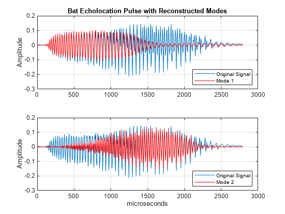
The ridges follow the time-varying nature of the modulated pulses. Reconstruct the signal modes by inverting the synchrosqueezed transform.

xrec = iwsst(sst,iridge);
subplot(2,1,1)
plot(time.*1e6,batsignal)
hold on
plot(time.*1e6,xrec(:,1),"r")
grid on
ylabel("Amplitude")
title("Bat Echolocation Pulse with Reconstructed Modes")
legend("Original Signal","Mode 1",Location="SouthEast")
subplot(2,1,2)
plot(time.*1e6,batsignal)
hold on
grid on
plot(time.*1e6,xrec(:,2),"r")
xlabel("microseconds")
ylabel("Amplitude")
legend("Original Signal","Mode 2",Location="SouthEast")

Figure contains 2 axes objects. Axes object 1 with title Bat Echolocation Pulse with Reconstructed Modes, ylabel Amplitude contains 2 objects of type line. These objects represent Original Signal, Mode 1. Axes object 2 with xlabel microseconds, ylabel Amplitude contains 2 objects of type line. These objects represent Original Signal, Mode 2.

You see that synchrosqueezing has extracted the two modes. If you sum the two dominant modes at each point in time, you essentially recover the entire echolocation pulse. In this application, synchrosqueezing allows you to isolate signal components where a traditional bandpass filter would fail.

Penalty Term in Ridge Extraction

The previous mode extraction example used a penalty term in the ridge extraction without explanation.

When you extract multiple ridges, or you have a single modulated component in additive noise, it is important to use a penalty term in the ridge extraction. The penalty term serves to prevent jumps in frequency as the region of highest energy in the time-frequency plane moves.

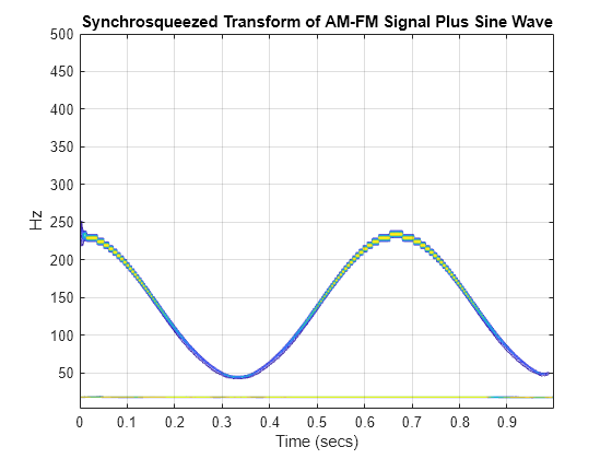
To demonstrate this, consider a two-component signal consisting of an amplitude and frequency-modulated signal plus a sine wave. The signal is sampled at 1000 Hz. The sine wave frequency is 18 Hz. The AM-FM signal is defined by:

$(2 + \cos (4 π t)) \sin (2 π 231 t + 90 \sin (3 π t))$

Load the signal and obtain the synchrosqueezed transform.

load multicompsig
sig = sig1+sig2;
[sst,f] = wsst(sig,sampfreq);
figure
contour(t,f,abs(sst))
grid on
title("Synchrosqueezed Transform of AM-FM Signal Plus Sine Wave")
xlabel("Time (secs)")
ylabel("Hz")

Figure contains an axes object. The axes object with title Synchrosqueezed Transform of AM-FM Signal Plus Sine Wave, xlabel Time (secs), ylabel Hz contains an object of type contour.

First attempt to extract two ridges from the synchrosqueezed transform without using a penalty.

[fridge,~] = wsstridge(sst,f,NumRidges=2);
hold on
plot(t,fridge,"k--",linewidth=2)

Figure contains an axes object. The axes object with title Synchrosqueezed Transform of AM-FM Signal Plus Sine Wave, xlabel Time (secs), ylabel Hz contains 3 objects of type contour, line.

You see that the ridge jumps between the AM-FM signal and the sine wave as the region of highest energy in the time-frequency plane changes between the two signals. Add a penalty term of 5 to the ridge extraction. In this case, jumps in frequency are penalized by a factor of 5 times the distance between the frequencies in terms of bins (not actual frequency in hertz).

[fridge,iridge] = wsstridge(sst,5,f,NumRidges=2);
figure
contour(t,f,abs(sst))
grid on
title("Synchrosqueezed Transform of AM-FM Signal Plus Sine Wave")
xlabel("Time (secs)")
ylabel("Hz")
hold on
plot(t,fridge,"k--",linewidth=2)
hold off

Figure contains an axes object. The axes object with title Synchrosqueezed Transform of AM-FM Signal Plus Sine Wave, xlabel Time (secs), ylabel Hz contains 3 objects of type contour, line.

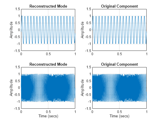
With the penalty term, the two modes of oscillation are isolated in two separate ridges. Reconstruct the modes along the time-frequency ridges from the synchrosqueezed transform.

xrec = iwsst(sst,iridge);

Plot the reconstructed modes along with the original signals for comparison.

subplot(2,2,1)
plot(t,xrec(:,1))
grid on
ylabel("Amplitude")
title("Reconstructed Mode")
ylim([-1.5 1.5])
subplot(2,2,2)
plot(t,sig2)
grid on
ylabel("Amplitude")
title("Original Component")
ylim([-1.5 1.5])
subplot(2,2,3)
plot(t,xrec(:,2))
grid on
xlabel("Time (secs)")
ylabel("Amplitude")
title("Reconstructed Mode")
ylim([-1.5 1.5])
subplot(2,2,4)
plot(t,sig1)
grid on
xlabel("Time (secs)")
ylabel("Amplitude")
title("Original Component")
ylim([-1.5 1.5])

Conclusions

In this example, you learned how to use wavelet synchrosqueezing to obtain a higher-resolution time-frequency analysis.

You also learned how to identify maxima ridges in the synchrosqueezed transform and reconstruct the time waveforms corresponding to those modes. Mode extraction from the synchrosqueezing transform can help you isolate signal components, which are difficult or impossible to isolate with conventional bandpass filtering.

Appendix

These helper functions are used in this example:

References

[1] Daubechies, Ingrid, Jianfeng Lu, and Hau-Tieng Wu. “Synchrosqueezed Wavelet Transforms: An Empirical Mode Decomposition-like Tool.” Applied and Computational Harmonic Analysis 30, no. 2 (March 2011): 243–61. https://doi.org/10.1016/j.acha.2010.08.002.

[2] Thakur, Gaurav, Eugene Brevdo, Neven S. Fučkar, and Hau-Tieng Wu. “The Synchrosqueezing Algorithm for Time-Varying Spectral Analysis: Robustness Properties and New Paleoclimate Applications.” Signal Processing 93, no. 5 (May 2013): 1079–94. https://doi.org/10.1016/j.sigpro.2012.11.029.

[3] Meignen, S., T. Oberlin, and S. McLaughlin. “A New Algorithm for Multicomponent Signals Analysis Based on SynchroSqueezing: With an Application to Signal Sampling and Denoising.” IEEE Transactions on Signal Processing 60, no. 11 (November 2012): 5787–98. https://doi.org/10.1109/TSP.2012.2212891.