Translation Invariant Wavelet Denoising with Cycle Spinning

Cycle spinning compensates for the lack of shift invariance in the critically-sampled wavelet transform by averaging over denoised cyclically-shifted versions of the signal or image. The appropriate inverse circulant shift operator is applied to the denoised signal/image and the results are averaged together to obtain the final denoised signal/image.

There are N unique cyclically-shifted versions of a signal of length, N. For an M-by-N image, there are MN versions. This makes using all possible shifted versions computationally prohibitive. However, in practice, good results can be obtained by using a small subset of the possible circular shifts.

The following example shows how you use wdenoise and circshift to denoise a 1-D signal using cycle spinning. For denoising grayscale and RGB images, wdenoise2 supports cycle spinning.

1-D Cycle Spinning

Open Live Script

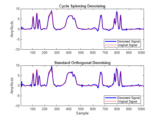
This example shows how to denoise a 1-D signal using cycle spinning and the shift-variant orthogonal nonredundant wavelet transform. The example compares the results of the two denoising methods.

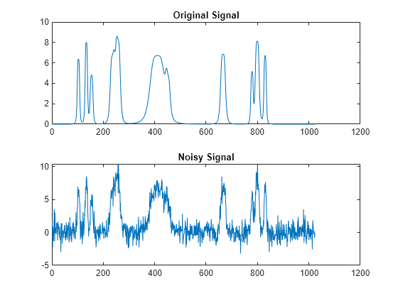
Create a noisy 1-D bumps signal with a signal-to-noise ratio of 6. The signal-to-noise ratio is defined as $\frac{N | | X | | \binom{2}{2}}{σ}$ where $N$ is the length of the signal, $| | X | | \binom{2}{2}$ is the squared L2 norm, and $σ^{2}$ is the variance of the noise.

rng default
[X,XN] = wnoise('bumps',10,sqrt(6));
subplot(2,1,1)
plot(X)
title('Original Signal')
subplot(2,1,2)
plot(XN)
title('Noisy Signal')

Figure contains 2 axes objects. Axes object 1 with title Original Signal contains an object of type line. Axes object 2 with title Noisy Signal contains an object of type line.

Denoise the signal using cycle spinning with 15 shifts, 7 to the left and 7 to the right, including the zero-shifted signal. Use wdenoise with default settings. By default, wdenoise uses Daubechies' least-asymmetric wavelet with four vanishing moments, sym4. Denoising is down to the minimum of floor(log2(N)) and wmaxlev(N,'sym4') where N is the number of samples in the data.

ydenoise = zeros(length(XN),15);
for nn = -7:7
    yshift = circshift(XN,[0 nn]);
    [yd,cyd] = wdenoise(yshift);
    ydenoise(:,nn+8) = circshift(yd,[0, -nn]);
end
ydenoise = mean(ydenoise,2);

Denoise the signal using wdenoise. Compare with the cycle spinning results.

xd = wdenoise(XN);
subplot(2,1,1)
plot(ydenoise,'b','linewidth',2)
hold on
plot(X,'r')
axis([1 1024 -10 10])
legend('Denoised Signal','Original Signal','Location','SouthEast')
ylabel('Amplitude')
title('Cycle Spinning Denoising')
hold off
subplot(2,1,2)
plot(xd,'b','linewidth',2)
hold on
plot(X,'r')
axis([1 1024 -10 10])
legend('Denoised Signal','Original Signal','Location','SouthEast')
xlabel('Sample')
ylabel('Amplitude')
title('Standard Orthogonal Denoising')
hold off

Figure contains 2 axes objects. Axes object 1 with title Cycle Spinning Denoising, ylabel Amplitude contains 2 objects of type line. These objects represent Denoised Signal, Original Signal. Axes object 2 with title Standard Orthogonal Denoising, xlabel Sample, ylabel Amplitude contains 2 objects of type line. These objects represent Denoised Signal, Original Signal.

absDiffDWT = norm(X-xd,2)

absDiffDWT = 
12.4248

absDiffCycleSpin = norm(X-ydenoise',2)

absDiffCycleSpin = 
10.6124

Cycle spinning with only 15 shifts has reduced the approximation error.

Translation Invariant Wavelet Denoising with Cycle Spinning

1-D Cycle Spinning

See Also

Functions

Apps