Main Content

wdenoise2

Wavelet image denoising

Description

example

IMDEN = wdenoise2(IM) denoises the grayscale or RGB image IM using an empirical Bayesian method. The bior4.4 wavelet is used with a posterior median threshold rule. Denoising is down to the minimum of floor(log2([M N])) and wmaxlev([M N],'bior4.4'), where M and N are the row and column sizes of the image. IMDEN is the denoised version of IM.

For RGB images, by default, wdenoise2 projects the image onto its principal component analysis (PCA) color space before denoising. To denoise an RGB image in the original color space, use the ColorSpace name-value pair.

IMDEN = wdenoise2(IM,LEVEL) denoises the image IM down to resolution level LEVEL. LEVEL is a positive integer less than or equal to floor(log2(min([M N]))), where M and N are the row and column sizes of the image.

[IMDEN,DENOISEDCFS] = wdenoise2(___) returns the scaling and denoised wavelet coefficients in DENOISEDCFS using any of the preceding syntaxes.

[IMDEN,DENOISEDCFS,ORIGCFS] = wdenoise2(___) returns the scaling and wavelet coefficients of the input image in ORIGCFS using any of the preceding syntaxes.

[IMDEN,DENOISEDCFS,ORIGCFS,S] = wdenoise2(___) returns the sizes of the approximation coefficients at the coarsest scale along with the sizes of the wavelet coefficients at all scales. S is a matrix with the same structure as the S output of wavedec2.

[IMDEN,DENOISEDCFS,ORIGCFS,S,SHIFTS] = wdenoise2(___) returns the shifts along the row and column dimensions for cycle spinning. SHIFTS is 2-by-(numshifts+1)2 matrix where each column of SHIFTS contains the shifts along the row and column dimension used in cycle spinning and numshifts is the value of CycleSpinning.

example

[___] = wdenoise2(___,Name,Value) returns the denoised image with additional options specified by one or more Name,Value pair arguments, using any of the preceding syntaxes.

wdenoise2(___) with no output arguments plots the original image along with the denoised image in the current figure.

Examples

collapse all

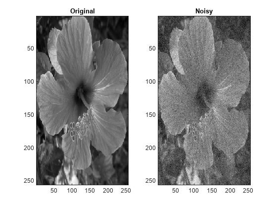
Load the structure flower. The structure contains a grayscale image of a flower, and a noisy version of that image. Display the original and noisy images.

load flower
subplot(1,2,1)
imagesc(flower.Orig)
title('Original')
subplot(1,2,2)
imagesc(flower.Noisy)
title('Noisy')
colormap gray

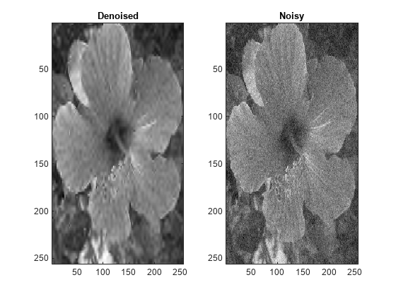
Denoise the noisy image using the default wdenoise2 settings. Compare with the original image.

imden = wdenoise2(flower.Noisy);
subplot(1,2,1)
imagesc(imden)
title('Denoised')
subplot(1,2,2)
imagesc(flower.Noisy)
title('Noisy')
colormap gray

Note the improvement in SNR before and after denoising.

beforeSNR = ...
    20*log10(norm(flower.Orig(:))/norm(flower.Orig(:)-flower.Noisy(:)))
beforeSNR = 14.1300
afterSNR = ...
    20*log10(norm(flower.Orig(:))/norm(flower.Orig(:)-imden(:)))
afterSNR = 20.1388

This example shows how to denoise a color image using cycle spinning.

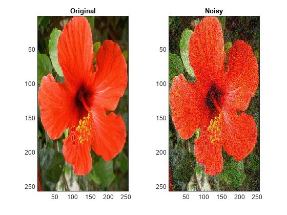
Load the structure colorflower. The structure contains the RGB image of a flower, and a noisy version of that image. Display the original and noisy images.

load colorflower
orig = colorflower.Orig;
noisy = colorflower.Noisy;
tiledlayout(1,2)
nexttile
imagesc(orig)
title('Original')
nexttile
imagesc(noisy)
title('Noisy')

Denoise the image down to level 2 using the default Bayesian method and cycle spinning with(1+1)2 shifts. Display the noisy and denoised images.

imden = wdenoise2(noisy,2,'CycleSpinning',1);
figure
tiledlayout(1,2)
nexttile
imagesc(imden)
title('Denoised')
nexttile
imagesc(noisy)
title('Noisy')

Compute the SNR before and after denoising.

beforeSNR = ...
    20*log10(norm(orig(:))/norm(orig(:)-noisy(:)))
beforeSNR = 11.2217
afterSNR = ...
    20*log10(norm(orig(:))/norm(orig(:)-imden(:)))
afterSNR = 19.8813

This example shows how to denoise an image using a specific subband to estimate the variance of the noise.

Load the structure flower. The structure contains the grayscale image of a flower, and a noisy version of that image. Display the original and noisy images.

load flower
subplot(1,2,1)
imagesc(flower.Orig)
title('Original')
subplot(1,2,2)
imagesc(flower.Noisy)
title('Noisy')
colormap gray

Denoise the image down to level 2 using the False Discovery Rate method with a Q-value of 0.01. Denoise only based on the diagonal wavelet coefficients. Display the denoised and noisy images.

imden = wdenoise2(flower.Noisy,2,...
    'DenoisingMethod',{'FDR',0.01},...
    'NoiseDirection',"d");
figure
subplot(1,2,1)
imagesc(imden)
title('Denoised')
subplot(1,2,2)
imagesc(flower.Noisy)
title('Noisy')
colormap gray

Compute the SNR before and after denoising.

beforeSNR = ...
    20*log10(norm(flower.Orig(:))/norm(flower.Orig(:)-flower.Noisy(:)))
beforeSNR = 14.1300
afterSNR = ...
    20*log10(norm(flower.Orig(:))/norm(flower.Orig(:)-imden(:)))
afterSNR = 19.9164

Input Arguments

collapse all

Input image to denoise, specified as a real-valued 2-D matrix or real-valued 3-D array. If IM is 3-D, IM is assumed to be a color image in the RGB color space and the third dimension of IM must be 3. For RGB images, wdenoise2 by default projects the image onto its PCA color space before denoising. To denoise an RGB image in the original color space, use the ColorSpace name-value pair.

Wavelet decomposition level used for denoising, specified as a positive integer. LEVEL is a positive integer less than or equal to floor(log2(min([M N]))), where M and N are the row and column sizes of the image. If unspecified, LEVEL defaults to min([floor(log2(min([M N]))),wmaxlev([M N],wname)]), where wname is the wavelet used ('bior4.4' by default).

Name-Value Arguments

Specify optional pairs of arguments as Name1=Value1,...,NameN=ValueN, where Name is the argument name and Value is the corresponding value. Name-value arguments must appear after other arguments, but the order of the pairs does not matter.

Before R2021a, use commas to separate each name and value, and enclose Name in quotes.

Example: 'NoiseEstimate','LevelDependent','Wavelet','sym6'

Wavelet, specified as a character vector or string scalar. The wavelet must be orthogonal or biorthogonal. Orthogonal and biorthogonal wavelets are designated as type 1 and type 2 wavelets respectively in the wavelet manager, wavemngr.

  • Valid built-in orthogonal wavelet families are: Best-localized Daubechies ("bl"), Beylkin ("beyl"), Coiflets ("coif"), Daubechies ("db"), Fejér-Korovkin ("fk"), Haar ("haar"), Han linear-phase moments ("han"), Morris minimum-bandwidth ("mb"), Symlets ("sym"), and Vaidyanathan ("vaid").

  • Valid built-in biorthogonal wavelet families are: Biorthogonal Spline ("bior"), and Reverse Biorthogonal Spline ("rbio").

For a list of wavelets in each family, see wfilters. You can also use waveinfo with the wavelet family short name. For example, waveinfo("db"). Use wavemngr("type",wn) to determine if the wavelet wn is orthogonal (returns 1) or biorthogonal (returns 2). For example, wavemngr("type","db6") returns 1.

Denoising method to use to determine the denoising thresholds for the image IM.

  • Bayes - Empirical Bayes

    This method uses a threshold rule based on assuming measurements have independent prior distributions given by a mixture model. Because measurements are used to estimate the weight in the mixture model, the method tends to work better with more samples. By default, the posterior median rule is used to measure risk [7].

  • FDR - False Discovery Rate

    This method uses a threshold rule based on controlling the expected ratio of false positive detections to all positive detections. The FDR method works best with sparse data. Choosing a ratio, or Q-value, less than 1/2 yields an asymptotically minimax estimator [1].

    Note

    For 'FDR', there is an optional argument for the Q-value, which is the proportion of false positives. Q is a real-valued scalar between 0 and 1/2, 0 < Q <= 1/2. To specify 'FDR' with a Q-value, use a cell array where the second element is the Q-value. For example, 'DenoisingMethod',{'FDR',0.01}. If unspecified, Q defaults to 0.05.

  • Minimax - Minimax Estimation

    This method uses a fixed threshold chosen to yield minimax performance for mean squared error against an ideal procedure. The minimax principle is used in statistics to design estimators. See thselect for more information.

  • SURE - Stein's Unbiased Risk Estimate

    This method uses a threshold selection rule based on Stein’s Unbiased Estimate of Risk (quadratic loss function). One gets an estimate of the risk for a particular threshold value (t). Minimizing the risks in (t) gives a selection of the threshold value.

  • UniversalThreshold - Universal Threshold 2ln(length(x)).

    This method uses a fixed-form threshold yielding minimax performance multiplied by a small factor proportional to log(length(X)).

Threshold rule to use to shrink the wavelet coefficients. 'ThresholdRule' is valid for all denoising methods, but the valid options and defaults depend on the denoising method. Rules possible for different denoising methods are specified as follows:

  • 'SURE', 'Minimax', 'UniversalThreshold': Valid options are 'Soft' or 'Hard'. The default is 'Soft'.

  • 'Bayes': Valid options are 'Median', 'Mean', 'Soft', or 'Hard'. The default is 'Median'.

  • 'FDR': The only supported option is 'Hard'. You do not need to define 'ThresholdRule' for 'FDR'

Method of estimating variance of noise in the image. Valid options are 'LevelIndependent' and 'LevelDependent'.

  • 'LevelIndependent' estimates the variance of the noise based on the finest-scale (highest-resolution) wavelet coefficients.

  • 'LevelDependent' estimates the variance of the noise based on the wavelet coefficients at each resolution level.

There are three wavelet subbands: horizontal, vertical, and diagonal. The value of 'NoiseDirection' specifies which subbands to use in estimating the variance.

Wavelet subbands to use to estimate the variance of the noise, specified as a string vector or scalar string. Valid entries are "h", "v", or "d", for the horizontal, vertical, and diagonal subbands, respectively.

Example: 'NoiseDirection',["h" "v"] specifies the horizontal and vertical subbands.

Number of circular shifts in both the row and column directions to use for denoising IM with cycle spinning. In cycle spinning, circular shifts of the image along the row and column dimensions are denoised, shifted back, and averaged together to provide the final result.

Generally, SNR improvements are observed with cycle spinning up to 3-4 shifts and asymptote after that. Because of the asymptotic effect on SNR and the fact that (CycleSpinning+1)2 images are being denoised, it is recommended to start with CycleSpinning equal to 0. Then gradually increase the number of shifts to determine if there is any improvement in SNR to justify the computational expense.

For example, specifying 'CycleSpinning',1 results in four copies of IM being denoised:

  • The original image (unshifted)

  • IM circularly shifted a single-element along the row dimension

  • IM circularly shifted a single-element along the column dimension

  • IM circularly shifted a single-element along both the row and column dimensions

The four denoised copies of IM are denoised, reconstructed, shifted back to their original positions, and averaged together. The value of CycleSpinning represents the maximum shift along both the row and column dimensions. For RGB images, there are no shifts applied along the color space dimension.

Color space used for denoising an RGB image. Valid options are 'PCA' and 'Original'.

  • 'PCA': The RGB image is first projected onto its PCA color space, denoised in the PCA color space, and returned to the original color space after denoising.

  • 'Original': Denoising is done in the same color space as the input image.

ColorSpace is valid only for RGB images.

Output Arguments

collapse all

Denoised image, returned as a matrix. The dimensions of IM and IMDEN are equal.

Scaling and denoised wavelet coefficients of the denoised image, returned as a real-valued matrix. DENOISEDCFS is a (numshifts+1)2-by-N matrix where N is the number of wavelet coefficients in the decomposition of IM and numshifts is the value of 'CycleSpinning'. Each row of DENOISEDCFS contains the denoised wavelet coefficients for one of (numshifts+1)2 shifted versions of IM. For RGB images, DENOISEDCFS are the denoised coefficients in the specified color space.

The ith row of DENOISEDCFS contains the denoised wavelet coefficients of the image circularly shifted by the amount returned in the ith column of SHIFTS. For example, if the second column of SHIFTS is [1 ; 1], the second row of DENOISEDCFS contains the denoised coefficients of the image circularly shifted by a single element in the row direction and a single element in the column direction.

Scaling and wavelet coefficients of the input image, returned as a real-valued 2-D matrix. ORIGCFS is a (numshifts+1)2-by-N matrix where N is the number of wavelet coefficients in the decomposition of IM and numshifts is the value of the 'CycleSpinning'. Each row of ORIGCFS contains the wavelet coefficients for one of (numshifts+1)2 shifted versions of IM. For RGB images, ORIGCFS are the original coefficients in the specified color space.

The ith row of ORIGCFS contains the wavelet coefficients of the image circularly shifted by the amount returned in the ith column of SHIFTS. For example, if the second column of SHIFTS is [1 ; 1], the second row of ORIGCFS contains the coefficients of the image circularly shifted by a single element in the row direction and a single element in the column direction.

Bookkeeping matrix. The matrix S contains the dimensions of the approximation coefficients at the coarsest scale, the sizes of the wavelet coefficients at all scales, and the size of the original input image. S is a matrix with the same structure as the S output of wavedec2.

Image shifts used in cycle spinning, returned as an integer-valued matrix. SHIFTS is 2-by-(numshifts+1)2 matrix where each column of SHIFTS contains the shifts along the row and column dimension used in cycle spinning.

References

[1] Abramovich, F., Y. Benjamini, D. L. Donoho, and I. M. Johnstone. “Adapting to Unknown Sparsity by Controlling the False Discovery Rate.” Annals of Statistics, Vol. 34, Number 2, pp. 584–653, 2006.

[2] Antoniadis, A., and G. Oppenheim, eds. Wavelets and Statistics. Lecture Notes in Statistics. New York: Springer Verlag, 1995.

[3] Donoho, D. L. “Progress in Wavelet Analysis and WVD: A Ten Minute Tour.” Progress in Wavelet Analysis and Applications (Y. Meyer, and S. Roques, eds.). Gif-sur-Yvette: Editions Frontières, 1993.

[4] Donoho, D. L., I. M. Johnstone. “Ideal Spatial Adaptation by Wavelet Shrinkage.” Biometrika, Vol. 81, pp. 425–455, 1994.

[5] Donoho, D. L. “De-noising by Soft-Thresholding.” IEEE Transactions on Information Theory, Vol. 42, Number 3, pp. 613–627, 1995.

[6] Donoho, D. L., I. M. Johnstone, G. Kerkyacharian, and D. Picard. “Wavelet Shrinkage: Asymptopia?” Journal of the Royal Statistical Society, series B, Vol. 57, No. 2, pp. 301–369, 1995.

[7] Johnstone, I. M., and B. W. Silverman. “Needles and Straw in Haystacks: Empirical Bayes Estimates of Possibly Sparse Sequences.” Annals of Statistics, Vol. 32, Number 4, pp. 1594–1649, 2004.

Extended Capabilities

Version History

Introduced in R2019a

See Also

|