Two-Dimensional CWT of Noisy Pattern

Visualize Isotropic Wavelet

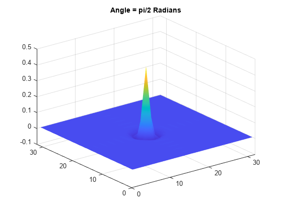
Use the isotropic (non-directional) Mexican hat wavelet, also known as the Ricker wavelet, and the anisotropic (directional) Morlet wavelet. Demonstrate that the real-valued Mexican hat wavelet does not depend on the angle.

Y = zeros(32,32);
Y(16,16) = 1;
cwtmexh = cwtft2(Y,wavelet="mexh",scales=1, ...
    angles=[0 pi/2]);
surf(real(cwtmexh.cfs(:,:,1,1,1)))
shading interp
title("Angle = 0 Radians")

Extract the wavelet corresponding to an angle of $$\pi$$/2 radians. The wavelet is isotropic and therefore does not differentiate oriented features in data.

surf(real(cwtmexh.cfs(:,:,1,1,2)))
shading interp
title("Angle = \pi/2 Radians")

Visualize Anisotropic Wavelet

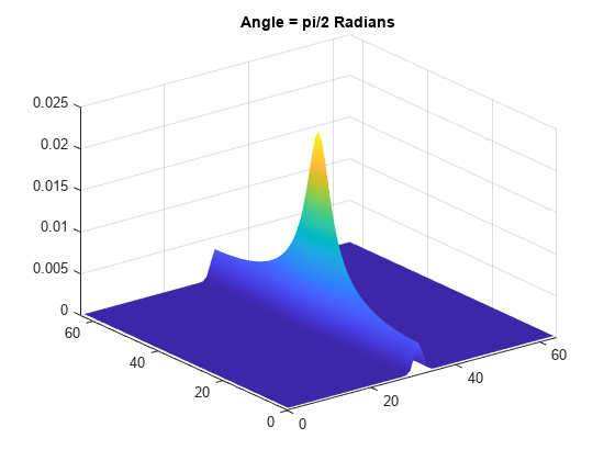
Repeat the preceding steps for the complex-valued Morlet wavelet. The Morlet wavelet has a larger spatial support than the Mexican hat wavelet, therefore this example uses a larger matrix. The wavelet is complex-valued, so the modulus is plotted.

Y = zeros(64,64);
Y(32,32) = 1;
cwtmorl = cwtft2(Y,wavelet="morl",scales=1, ...
    angles=[0 pi/2]);
surf(abs(cwtmorl.cfs(:,:,1,1,1)))
shading interp
title("Angle = 0 Radians")

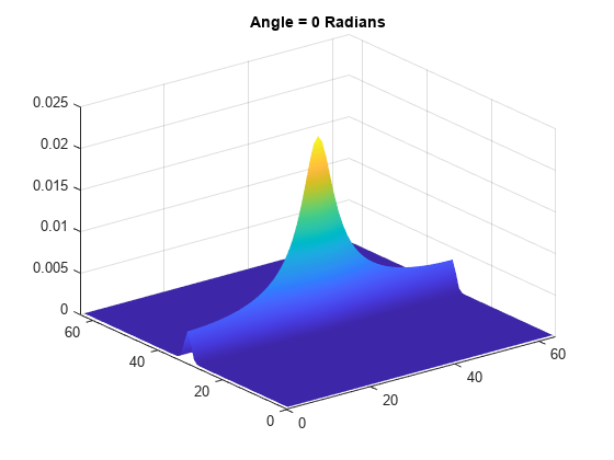
Extract the wavelet corresponding to an angle of $$\pi$$/2 radians. Unlike the Mexican hat wavelet, the Morlet wavelet is not isotropic and therefore is sensitive to the direction of features in the data.

surf(abs(cwtmorl.cfs(:,:,1,1,2)))
shading interp
title("Angle = \pi/2 Radians")

Detect Pattern

Apply the Mexican hat and Morlet wavelets to the detection of a pattern in noise. Create a pattern consisting of line segments joined at a 90-degree angle. The amplitude of the pattern is 3 and it occurs in additive N(0,1) white Gaussian noise.

X = zeros(256,256);
X(100:200,100:102) = 3;
X(200:202,100:125) = 3;
X = X+randn(size(X));
imagesc(X)
axis xy

Using Isotropic Wavelet

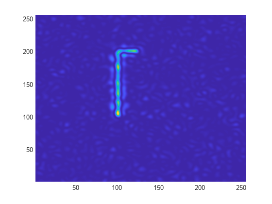
Obtain the 2-D CWT at scales 3 to 8 in 0.5 increments with the Mexican hat wavelet. Visualize the magnitude-squared 2-D wavelet coefficients at scale 3.

cwtmexh = cwtft2(X,wavelet="mexh",scales=3:0.5:8);
surf(abs(cwtmexh.cfs(:,:,1,3,1)).^2)
view(0,90)
shading interp
axis tight

Using Anisotropic Wavelet

Use a directional Morlet wavelet to extract the vertical and horizontal line segments separately. The vertical line segment is extracted by one angle. The horizontal line segment is extracted by another angle.

cwtmorl = cwtft2(X,wavelet="morl",scales=3:0.5:8, ...
    angles=[0 pi/2]);
surf(abs(cwtmorl.cfs(:,:,1,4,1)).^2)
view(0,90)
shading interp
axis tight

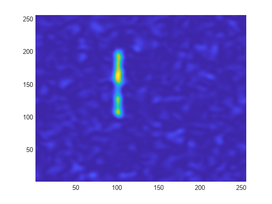
figure
surf(abs(cwtmorl.cfs(:,:,1,4,2)).^2)
view(0,90)
shading interp
axis tight