Wavelet Packets: Decomposing the Details

Discrete Wavelet and Discrete Wavelet Packet Transforms

The following figure shows a DWT tree for a 1-D input signal.

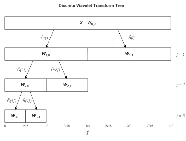
Figure 1: DWT Tree down to level 3 for a 1-D input signal.

$$\underset{}{\overset{\sim }{G}}(f)$$ is the scaling (lowpass) analysis filter and $$\underset{}{\overset{\sim }{H}}(f)$$ represents the wavelet (highpass) analysis filter. The labels at the bottom show the partition of the frequency axis [0,1/2] into subbands.

The figure shows that subsequent levels of the DWT operate only on the outputs of the lowpass (scaling) filter. At each level, the DWT divides the signal into octave bands. In the critically-sampled DWT, the outputs of the bandpass filters are downsampled by two at each level. In the undecimated discrete wavelet transform, the outputs are not downsampled.

Compare the DWT tree with the full wavelet packet tree.

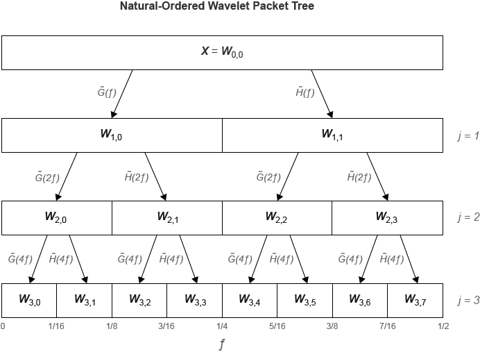
Figure 2: Full wavelet packet tree down to level 3.

In the wavelet packet transform, the filtering operations are also applied to the wavelet, or detail, coefficients. The result is that wavelet packets provide a subband filtering of the input signal into progressively finer equal-width intervals. At each level, $$j$$, the frequency axis [0,1/2] is divided into $$2^j$$ subbands. The subbands in hertz at level $$j$$ are approximately

$$[\frac{nFs}{2^{j+1}},\frac{(n+1)Fs}{2^{j+1}})n=0,1,\dots 2^j-1$$ where $$\text{Fs}$$ is the sampling frequency.

How good this bandpass approximation is depends on how frequency-localized the filters are. For Fejér-Korovkin filters like 'fk18' (18 coefficients), the approximation is quite good. For a filter like the Haar ('haar'), the approximation is not accurate.

In the critically-sampled wavelet packet transform the outputs of the bandpass filters are downsampled by two. In the undecimated wavelet packet transform, the outputs are not downsampled.

Time-Frequency Analysis with Wavelet Packets

Because wavelet packets divide the frequency axis into finer intervals than the DWT, wavelet packets are superior at time-frequency analysis. As an example, consider two intermittent sine waves with frequencies of 150 and 200 Hz in additive noise. The data are sampled at 1 kHz. To prevent the loss of time resolution inherent in the critically-sampled wavelet packet transform, use the undecimated transform.

dt = 0.001;
t = 0:dt:1-dt;
x = cos(2*pi*150*t).*(t>=0.2 & t<0.4) + ...
    sin(2*pi*200*t).*(t>0.6 & t<0.9);
y = x+0.05*randn(size(t));
[wpt,~,F] = modwpt(x,'TimeAlign',true);
contour(t,F.*(1/dt),abs(wpt).^2)
grid on
xlabel('Time (secs)')
ylabel('Hz')
title('Time-Frequency Analysis -- Undecimated Wavelet Packet Transform')

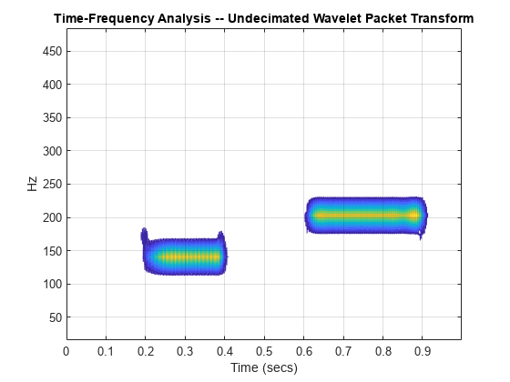
Note that the wavelet packet transform is able to separate the 150 and 200 Hz components. This is not true of the DWT, because 150 and 200 Hz fall in the same octave band. The octave bands for a level-four DWT are (in Hz)

Demonstrate that these two components are time-localized by the DWT but not separated in frequency.

mra  = modwtmra(modwt(y,'fk18',4),'fk18');
J = 5:-1:1;
freq = 1/2*(1000./2.^J);
contour(t,freq,flipud(abs(mra).^2))
grid on
ylim([0 500])
xlabel('Time (secs)')
ylabel('Hz')
title('Time-Frequency Analysis -- Undecimated Wavelet Transform')

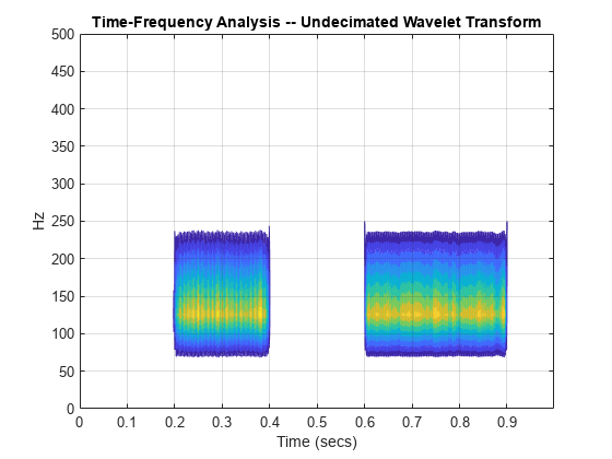
Of course, the continuous wavelet transform (CWT) provides a higher resolution time-frequency analysis than the wavelet packet transform, but wavelet packets have the added benefit of being an orthogonal transform (when using an orthogonal wavelet). An orthogonal transform means that the energy in the signal is preserved and partitioned among the coefficients as the next section demonstrates.

Energy Preservation in the Wavelet Packet Transform

In addition to filtering a signal into equal-width subbands at each level, the wavelet packet transform partitions the signal's energy among the subbands. This is true for both the decimated and undecimated wavelet packet transforms. To demonstrate this, load a dataset containing a seismic recording of an earthquake. This data is similar to the time series used in the signal classification example below.

load kobe
plot(kobe)
grid on
xlabel('Seconds')
title('Kobe Earthquake Data')
axis tight

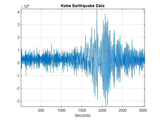
Obtain both the decimated and undecimated wavelet packet transforms of the data down to level 3. To ensure consistent results for the decimated wavelet packet transform, set the boundary extension mode to 'periodic'.

wptreeDecimated = dwpt(kobe,'Level',3,'Boundary','periodic');
wptUndecimated = modwpt(kobe,3);

Compute the total energy in both the decimated and undecimated wavelet packet level-three coefficients and compare to the energy in the original signal.

decimatedEnergy = sum(cell2mat(cellfun(@(x) sum(abs(x).^2),wptreeDecimated, ...
    'UniformOutput',false)))

decimatedEnergy = 
2.0189e+11

undecimatedEnergy = sum(sum(abs(wptUndecimated).^2,2))

undecimatedEnergy = 
2.0189e+11

signalEnergy = norm(kobe,2)^2

signalEnergy = 
2.0189e+11

The DWT shares this important property with the wavelet packet transform.

wt = modwt(kobe,'fk18',3);
undecimatedWTEnergy = sum(sum(abs(wt).^2,2))

undecimatedWTEnergy = 
2.0189e+11

Because the wavelet packet transform at each level divides the frequency axis into equal-width intervals and partitions the signal energy among those intervals, you can often construct useful feature vectors for classification just by retaining the relative energy in each wavelet packet. The next example demonstrates this.

Wavelet Packet Classification -- Earthquake or Explosion?

Seismic recordings pick up activity from many sources. It is important to be able to classify this activity based on its origin. For example, earthquakes and explosions may present similar time-domain signatures, but it is very important to differentiate between these two events. The dataset EarthQuakeExplosionData contains 16 recordings with 2048 samples. The first 8 recordings (columns) are seismic recordings of earthquakes, the last 8 recordings (columns) are seismic recordings of explosions. Load the data and plot an earthquake and explosion recording for comparison. The data is taken from the R package astsa Stoffer [4], which supplements Shumway and Stoffer [3]. The author has kindly allowed its use in this example.

Plot a time series from each group for comparison.

load EarthQuakeExplosionData
tiledlayout(2,1)
nexttile
plot(EarthQuakeExplosionData(:,3))
xlabel('Time')
title('Earthquake Recording')
grid on
axis tight
nexttile
plot(EarthQuakeExplosionData(:,9))
xlabel('Time')
title('Explosion Recording')
grid on
axis tight

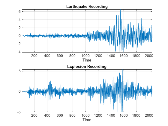
Form a wavelet packet feature vector by decomposing each time series down to level three using the 'fk6' wavelet with an undecimated wavelet packet transform. This results in 8 subbands with an approximate width of 1/16 cycles/sample. Use the relative energy in each subband to create a feature vector. As an example, obtain a wavelet packet relative energy feature vector for the first earthquake recording.

[wpt,~,F,E,RE] = modwpt(EarthQuakeExplosionData(:,1),3,'fk6');

RE contains the relative energy in each of the 8 subbands. If you sum all the elements in RE, it is equal to 1. Note that this is a significant reduction in data. A time series of length 2048 is reduced to a vector with 8 elements, each element representing the relative energy in the wavelet packet nodes at level 3. The helper function helperEarthQuakeExplosionClassifier obtains the relative energies for each of the 16 recordings at level 3 using the 'fk6' wavelet. This results in a 16-by-8 matrix and uses these feature vectors as inputs to a kmeans classifier. The classifier uses the Gap statistic criterion to determine the optimal number of clusters for the feature vectors between 1 and 6 and classifies each vector. Additionally, the classifier performs the exact same classification on the undecimated wavelet transform coefficients at level 3 obtained with the 'fk6' wavelet and power spectra for each of the time series. The undecimated wavelet transform results in a 16-by-4 matrix (3 wavelet subbands and 1 scaling subband). The power spectra result in a 16-by-1025 matrix. The source code for helperEarthQuakeExplosionClassifier is listed in the appendix. You must have Statistics and Machine Learning Toolbox™ and Signal Processing Toolbox™ to run the classifier.

Level = 3;
[WavPacketCluster,WtCluster,PspecCluster] = ...
helperEarthQuakeExplosionClassifier(EarthQuakeExplosionData,Level)

WavPacketCluster = 
  GapEvaluation with properties:

    NumObservations: 16
         InspectedK: [1 2 3 4 5 6]
    CriterionValues: [-0.0039 0.0779 0.1314 0.0862 0.0296 -0.0096]
           OptimalK: 2

WtCluster = 
  GapEvaluation with properties:

    NumObservations: 16
         InspectedK: [1 2 3 4 5 6]
    CriterionValues: [-0.0095 0.0474 0.0706 0.0260 -0.0280 -0.0346]
           OptimalK: 2

PspecCluster = 
  GapEvaluation with properties:

    NumObservations: 16
         InspectedK: [1 2 3 4 5 6]
    CriterionValues: [0.3786 0.3534 0.3456 0.2864 0.3271 0.3355]
           OptimalK: 1

WavPacketCluster is the clustering output for the undecimated wavelet packet feature vectors. WtCluster is the clustering output using the undecimated DWT feature vectors, and PspecCluster is the output for the clustering based on the power spectra. The wavelet packet classification has identified two clusters (OptimalK: 2) as the optimal number. Examine the results of the wavelet packet clustering.

res = [ WavPacketCluster.OptimalY(1:8)' ; WavPacketCluster.OptimalY(9:end)']

res = 2×8

     1     2     2     2     2     2     2     2
     1     1     1     1     1     1     1     2

You see that only two errors have been made. Of the eight earthquake recordings, seven are classified together (group 2) and one is mistakenly classified as belonging to group 1. The same is true of the 8 explosion recordings -- 7 are classified together and 1 is misclassified. Classifications based on the level-three undecimated DWT and power spectra return one cluster as the optimal solution.

If you repeat the above with the level equal to 4, the undecimated wavelet transform and wavelet packet transform perform identically. Both identify two clusters as optimal, and both misclassify the first and last time series as belonging to the other group.

Conclusions

In this example, you learned how the wavelet packet transform differs from the discrete wavelet transform. Specifically, the wavelet packet tree also filters the wavelet (detail) coefficients, while the wavelet transform only iterates on the scaling (approximation) coefficients.

You learned that the wavelet packet transform shares the important energy-preserving property of the DWT while providing superior frequency resolution. In some applications, this superior frequency resolution makes the wavelet packet transform an attractive alternative to the DWT.

Appendix

helperEarthQuakeExplosionClassifier

function [WavPacketCluster,WtCluster,PspecCluster] = helperEarthQuakeExplosionClassifier(Data,Level)  
%   This function is provided solely in support of the featured example
%   waveletpacketsdemo.mlx. 
%   This function may be changed or removed in a future release.
%   Data - The data matrix with individual time series as column vectors.
%   Level - The level of the wavelet packet and wavelet transforms

NP = 2^Level;
NW = Level+1;
WpMatrix = zeros(16,NP);
WtMatrix = zeros(16,NW);

for jj = 1:8
    [~,~,~,~,RE] = modwpt(Data(:,jj),Level,'fk6');
    wt = modwt(Data(:,jj),Level,'fk6');
    WtMatrix(jj,:) = sum(abs(wt).^2,2)./norm(Data(:,jj),2)^2;
    WpMatrix(jj,:) = RE;
end

for kk = 9:16
    [~,~,~,~,RE] = modwpt(Data(:,kk),Level,'fk6');
    wt = modwt(Data(:,kk),Level,'fk6');
    WtMatrix(kk,:) = sum(abs(wt).^2,2)./norm(Data(:,kk),2)^2;
    WpMatrix(kk,:) = RE;
end

% For repeatability
rng('default');

WavPacketCluster = evalclusters(WpMatrix,'kmeans','gap','KList',1:6,...
    'Distance','cityblock');

WtCluster = evalclusters(WtMatrix,'kmeans','gap','KList',1:6,...
'Distance','cityblock');

Pxx = periodogram(Data,hamming(numel(Data(:,1))),[],1,'power');

PspecCluster = evalclusters(Pxx','kmeans','gap','KList',1:6,...
    'Distance','cityblock');
end

References

[1] Wickerhauser, Mladen Victor. Adapted Wavelet Analysis from Theory to Software. Wellesley, MA: A.K. Peters, 1994.
[2] Percival, Donald B., and Andrew T. Walden. Wavelet Methods for Time Series Analysis. Cambridge Series in Statistical and Probabilistic Mathematics. Cambridge ; New York: Cambridge University Press, 2000.
[3] Shumway, Robert H., and David S. Stoffer. Time Series Analysis and Its Applications: With R Examples. 3rd ed. Springer Texts in Statistics. New York: Springer, 2011.
[4] Stoffer, D. H. "asta:
Applied Statistical Time Series Analysis." R package version 1.3.
https://CRAN.R-project.org/package=astsa,