主要内容
Results for
I was looking into the possibility of making a spin-to-win prize wheel in MATLAB. I was looking around, and if someone has made one before they haven't shared. A labeled colored spinning wheel, that would slow down and stop (or I would take just stopping) at a random spot each time. I would love any tips or links to helpful resources!
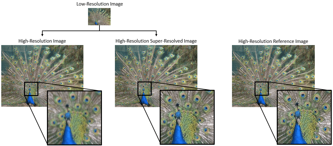
Many of the examples in the MATLAB documentation are extremely high quality articles, often worthy of attention in their own right. Time to start celebrating them! Today's is how to increase Image Resolution using deep learning
https://uk.mathworks.com/help/deeplearning/ug/single-image-super-resolution-using-deep-learning.html
MathWorks
Accelerating the pace of engineering and science.
It is easy to obtain sankey plot like that using my tool:
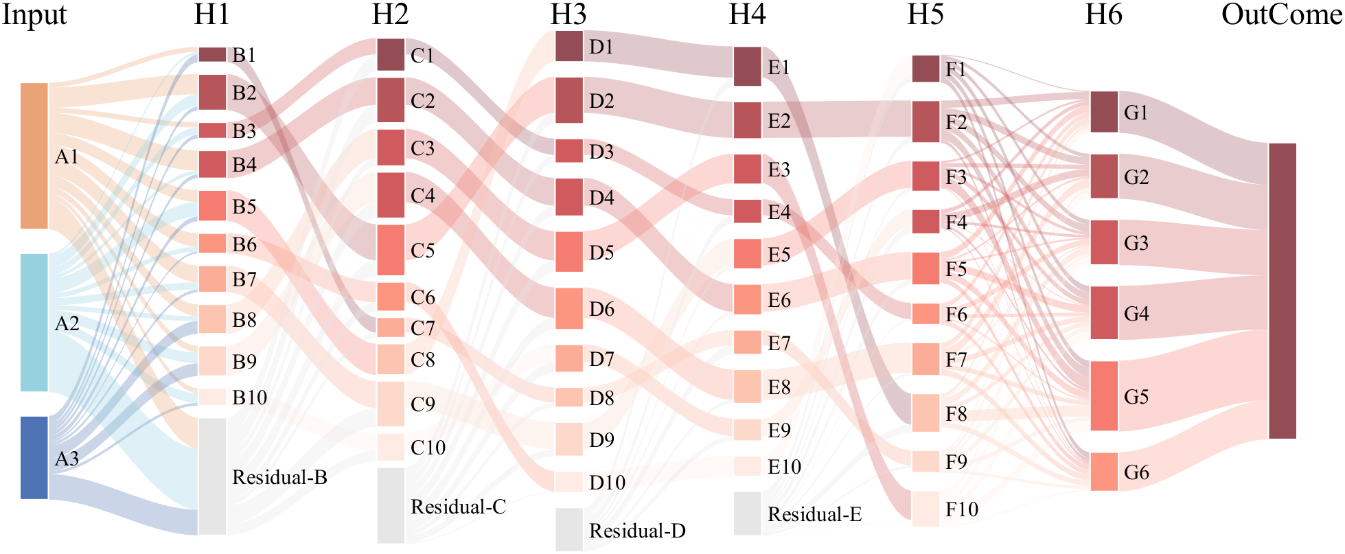
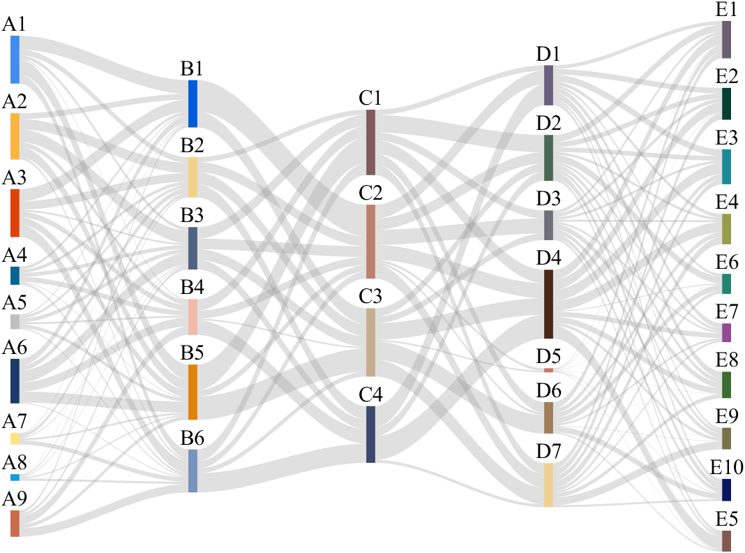
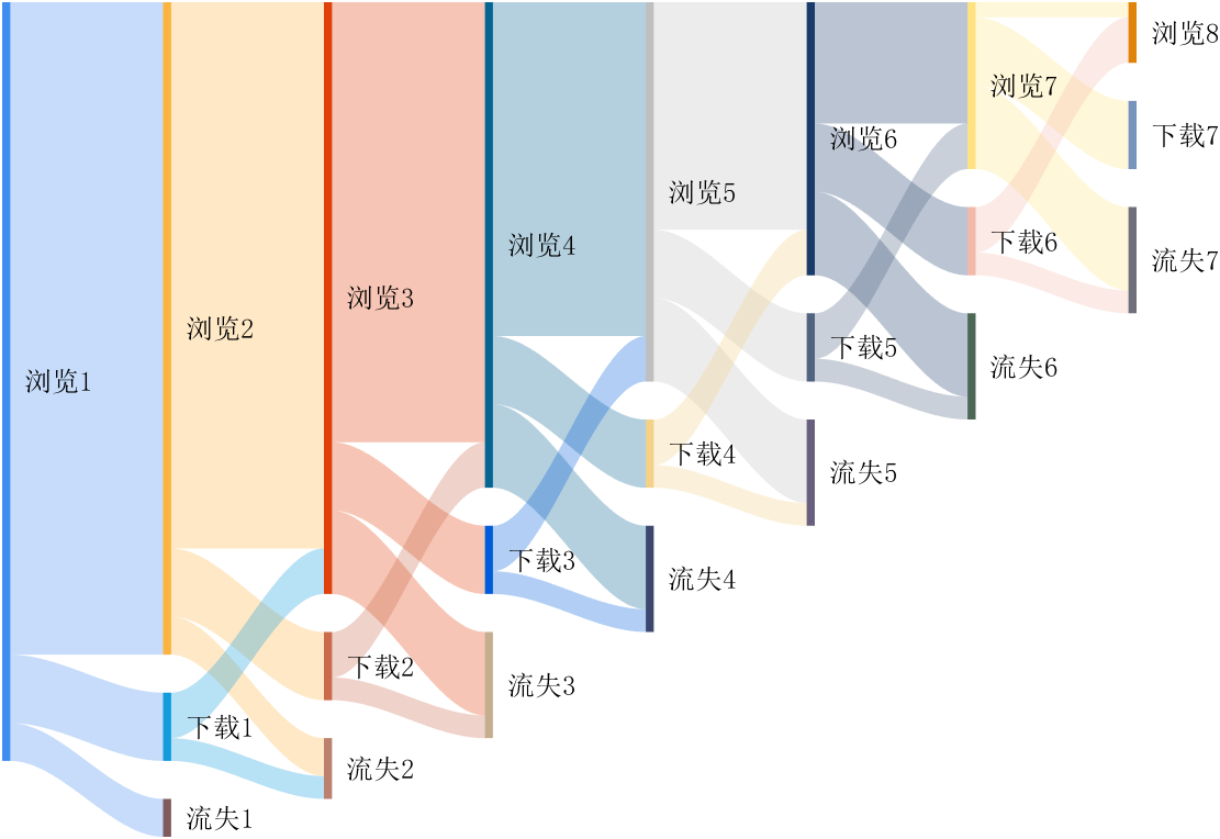
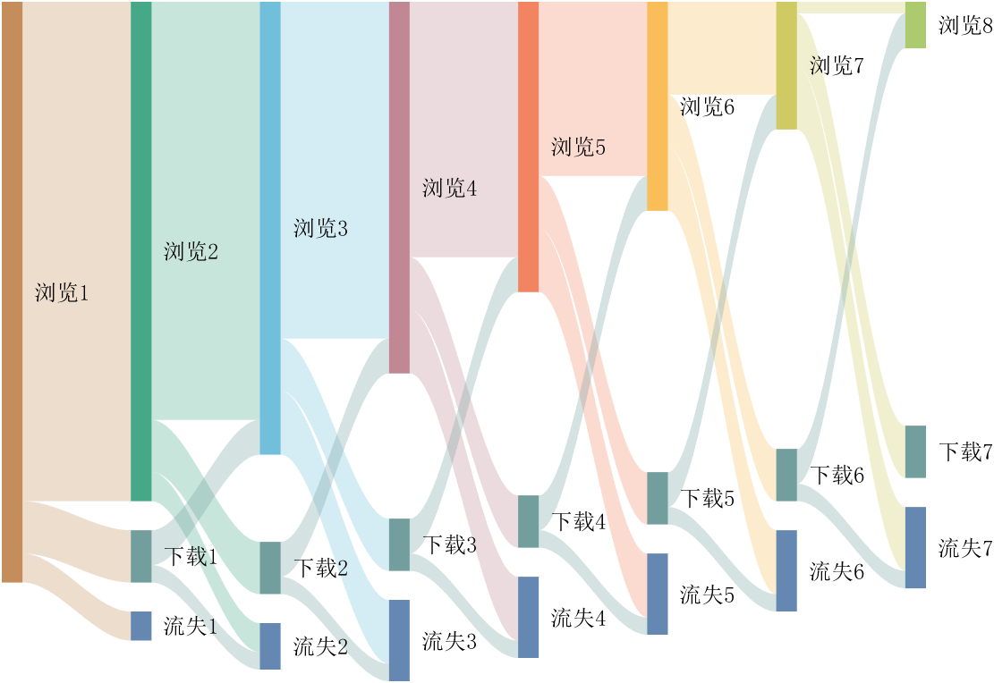
sankey plot
sankey plot /sankey diagram /sankey chart
code is here
You can also see the animated version of the competition here
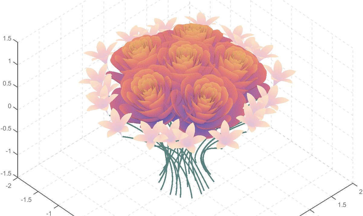
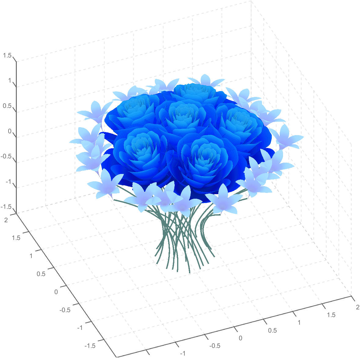
rose bouquet
rose bouquet by slandarer
Struct is an easy way to combine different types of variants. But now MATLAB supports classes well, and I think class is always a better alternative than struct. I can't find a single scenario that struct is necessary. There are many shortcomings using structs in a project, e.g. uncontrollable field names, unexamined values, etc. What's your opinion?
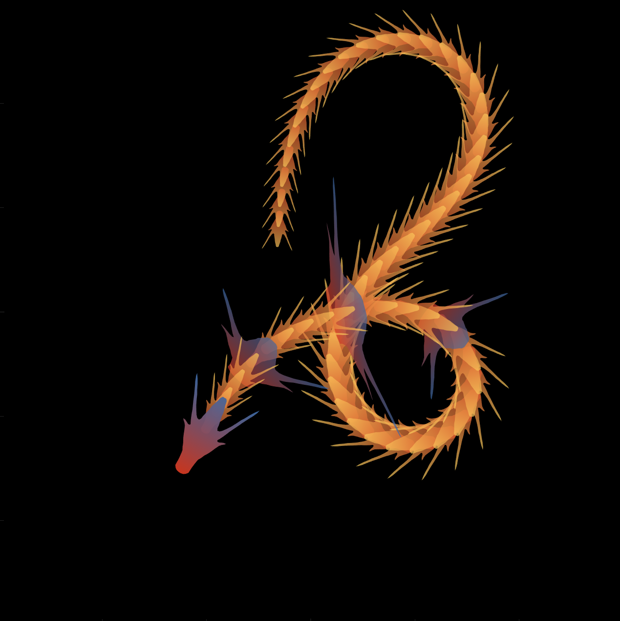
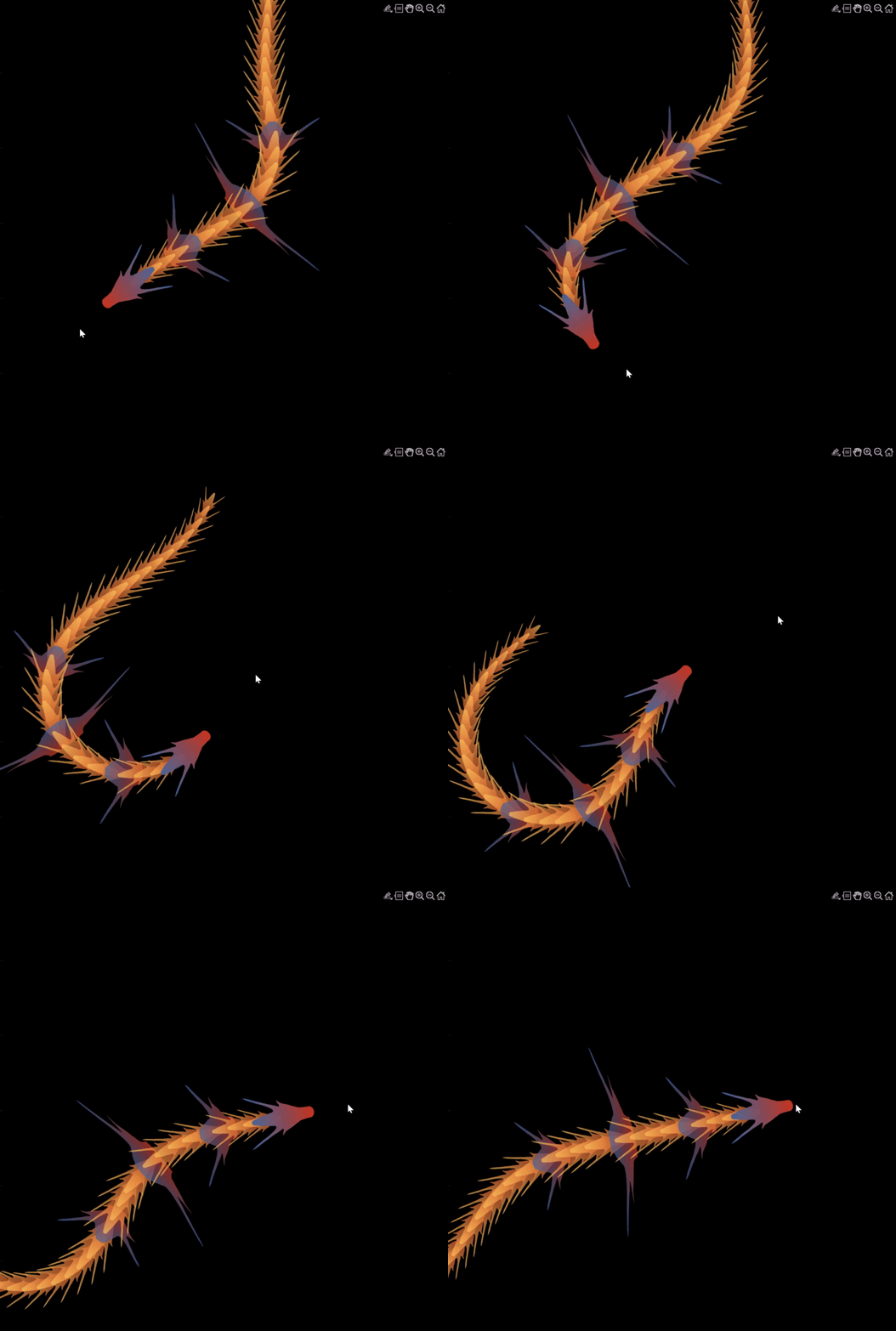
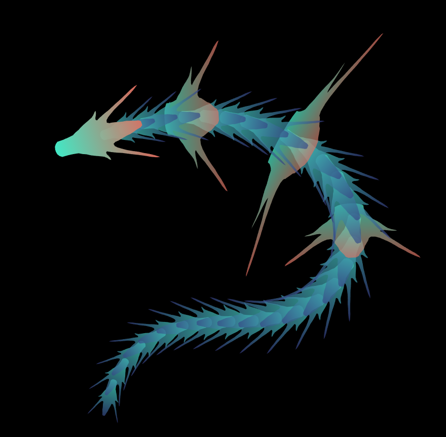
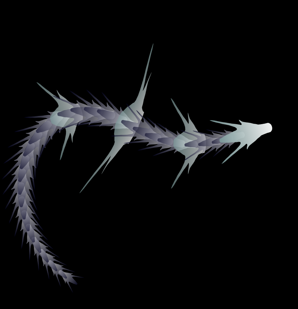
function dragon24
% Copyright (c) 2024, Zhaoxu Liu / slandarer
baseV=[ -.016,.822; -.074,.809; -.114,.781; -.147,.738; -.149,.687; -.150,.630;
-.157,.554; -.166,.482; -.176,.425; -.208,.368; -.237,.298; -.284,.216;
-.317,.143; -.338,.091; -.362,.037;-.382,-.006;-.420,-.051;-.460,-.084;
-.477,-.110;-.430,-.103;-.387,-.084;-.352,-.065;-.317,-.060;-.300,-.082;
-.331,-.139;-.359,-.201;-.385,-.262;-.415,-.342;-.451,-.418;-.494,-.510;
-.533,-.599;-.569,-.675;-.607,-.753;-.647,-.829;-.689,-.932;-.699,-.988;
-.639,-.905;-.581,-.809;-.534,-.717;-.489,-.642;-.442,-.543;-.393,-.447;
-.339,-.362;-.295,-.296;-.251,-.251;-.206,-.241;-.183,-.281;-.175,-.350;
-.156,-.434;-.136,-.521;-.128,-.594;-.103,-.677;-.083,-.739;-.067,-.813;-.039,-.852];
% 基础比例、上色方式数据
baseV=[0,.82;baseV;baseV(end:-1:1,:).*[-1,1];0,.82];
baseV=baseV-mean(baseV,1);
baseF=1:size(baseV,1);
baseY=baseV(:,2);
baseY=(baseY-min(baseY))./(max(baseY)-min(baseY));
N=30;
baseR=sin(linspace(pi/4,5*pi/6,N))./1.2;
baseR=[baseR',baseR'];baseR(1,:)=[1,1];
baseR(5,:)=[2,.6];
baseR(10,:)=[3.7,.4];
baseR(15,:)=[1.8,.6];
baseT=[zeros(N,1),ones(N,1)];
baseM=zeros(N,2);
baseD=baseM;
ratioT=@(Mat,t)Mat*[cos(t),sin(t);-sin(t),cos(t)];
% 配色数据
CList=[211,56,32;56,105,166;253,209,95]./255;
% CList=bone(4);CList=CList(2:4,:);
% CList=flipud(bone(3));
% CList=lines(3);
% CList=colorcube(3);
% CList=rand(3)
baseC1=CList(2,:)+baseY.*(CList(1,:)-CList(2,:));
baseC2=CList(3,:)+baseY.*(CList(1,:)-CList(3,:));
% 构建图窗
fig=figure('units','normalized','position',[.1,.1,.5,.8],...
'UserData',[98,121,32,115,108,97,110,100,97,114,101,114]);
axes('parent',fig,'NextPlot','add','Color',[0,0,0],...
'DataAspectRatio',[1,1,1],'XLim',[-6,6],'YLim',[-6,6],'Position',[0,0,1,1]);
% 构造龙每个部分句柄
dragonHdl(1)=patch('Faces',baseF,'Vertices',baseV,'FaceVertexCData',baseC1,'FaceColor','interp','EdgeColor','none','FaceAlpha',.95);disp(char(fig.UserData))
for i=2:N
dragonHdl(i)=patch('Faces',baseF,'Vertices',baseV.*baseR(i,:)-[0,i./2.5-.3],'FaceVertexCData',baseC2,'FaceColor','interp','EdgeColor','none','FaceAlpha',.7);
end
set(dragonHdl(5),'FaceVertexCData',baseC1,'FaceAlpha',.7)
set(dragonHdl(10),'FaceVertexCData',baseC1,'FaceAlpha',.7)
set(dragonHdl(15),'FaceVertexCData',baseC1,'FaceAlpha',.7)
for i=N:-1:1,uistack(dragonHdl(i),'top');end
for i=1:N
baseM(i,:)=mean(get(dragonHdl(i),'Vertices'),1);
end
baseD=diff(baseM(:,2));Pos=[0,2];
% 主循环及旋转、运动计算
set(gcf,'WindowButtonMotionFcn',@dragonFcn)
fps=8;
game=timer('ExecutionMode', 'FixedRate', 'Period',1/fps, 'TimerFcn', @dragonGame);
start(game)
% Copyright (c) 2023, Zhaoxu Liu / slandarer
set(gcf,'tag','co','CloseRequestFcn',@clo);
function clo(~,~)
stop(game);delete(findobj('tag','co'));clf;close
end
function dragonGame(~,~)
Dir=Pos-baseM(1,:);
Dir=Dir./norm(Dir);
baseT=(baseT(1:end,:)+[Dir;baseT(1:end-1,:)])./2;
baseT=baseT./(vecnorm(baseT')');
theta=atan2(baseT(:,2),baseT(:,1))-pi/2;
baseM(1,:)=baseM(1,:)+(Pos-baseM(1,:))./30;
baseM(2:end,:)=baseM(1,:)+[cumsum(baseD.*baseT(2:end,1)),cumsum(baseD.*baseT(2:end,2))];
for ii=1:N
set(dragonHdl(ii),'Vertices',ratioT(baseV.*baseR(ii,:),theta(ii))+baseM(ii,:))
end
end
function dragonFcn(~,~)
xy=get(gca,'CurrentPoint');
x=xy(1,1);y=xy(1,2);
Pos=[x,y];
Pos(Pos>6)=6;
Pos(Pos<-6)=6;
end
end
There will be a warning when we try to solve equations with piecewise:
syms x y
a = x+y;
b = 1.*(x > 0) + 2.*(x <= 0);
eqns = [a + b*x == 1, a - b == 2];
S = solve(eqns, [x y]);
% 错误使用 mupadengine/feval_internal
% System contains an equation of an unknown type.
%
% 出错 sym/solve (第 293 行)
% sol = eng.feval_internal('solve', eqns, vars, solveOptions);
%
% 出错 demo3 (第 5 行)
% S=solve(eqns,[x y]);
But I found that the solve function can include functions such as heaviside to indicate positive and negative:
syms x y
a = x+y;
b = floor(heaviside(x)) - 2*abs(2*heaviside(x) - 1) + 2*floor(-heaviside(x)) + 4;
eqns = [a + b*x == 1, a - b == 2];
S = solve(eqns, [x y])
% S =
% 包含以下字段的 struct:
%
% x: -3/2
% y: 11/2
The piecewise function is divided into two sections, which is so complex, so this work must be encapsulated as a function to complete:
function pwFunc=piecewiseSym(x,waypoint,func,pfunc)
% @author : slandarer
gSign=[1,heaviside(x-waypoint)*2-1];
lSign=[heaviside(waypoint-x)*2-1,1];
inSign=floor((gSign+lSign)/2);
onSign=1-abs(gSign(2:end));
inFunc=inSign.*func;
onFunc=onSign.*pfunc;
pwFunc=simplify(sum(inFunc)+sum(onFunc));
end
Function Introduction
- x : Argument
- waypoint : Segmentation point of piecewise function
- func : Functions on each segment
- pfunc : The value at the segmentation point
example
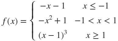
syms x
% x waypoint func pfunc
f=piecewiseSym(x,[-1,1],[-x-1,-x^2+1,(x-1)^3],[-x-1,(x-1)^3]);
For example, find the analytical solution of the intersection point between the piecewise function and f=0.4 and plot it:
syms x
% x waypoint func pfunc
f=piecewiseSym(x,[-1,1],[-x-1,-x^2+1,(x-1)^3],[-x-1,(x-1)^3]);
% solve
S=solve(f==.4,x)
% S =
%
% -7/5
% (2^(1/3)*5^(2/3))/5 + 1
% -15^(1/2)/5
% 15^(1/2)/5
% draw
xx=linspace(-2,2,500);
f=matlabFunction(f);
yy=f(xx);
plot(xx,yy,'LineWidth',2);
hold on
scatter(double(S),.4.*ones(length(S),1),50,'filled')
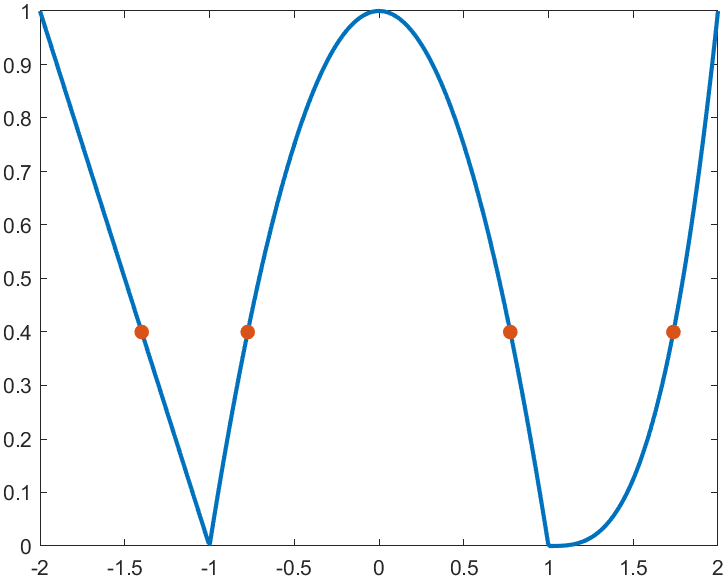
precedent
syms x y
a=x+y;
b=piecewiseSym(x,0,[2,1],2);
eqns = [a + b*x == 1, a - b == 2];
S=solve(eqns,[x y])
% S =
% 包含以下字段的 struct:
%
% x: -3/2
% y: 11/2
It is pretty easy to draw a cool heatmap for I have uploaded a tool to fileexchange:
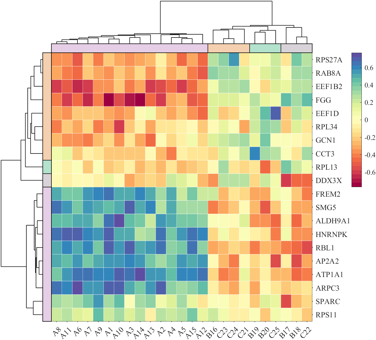
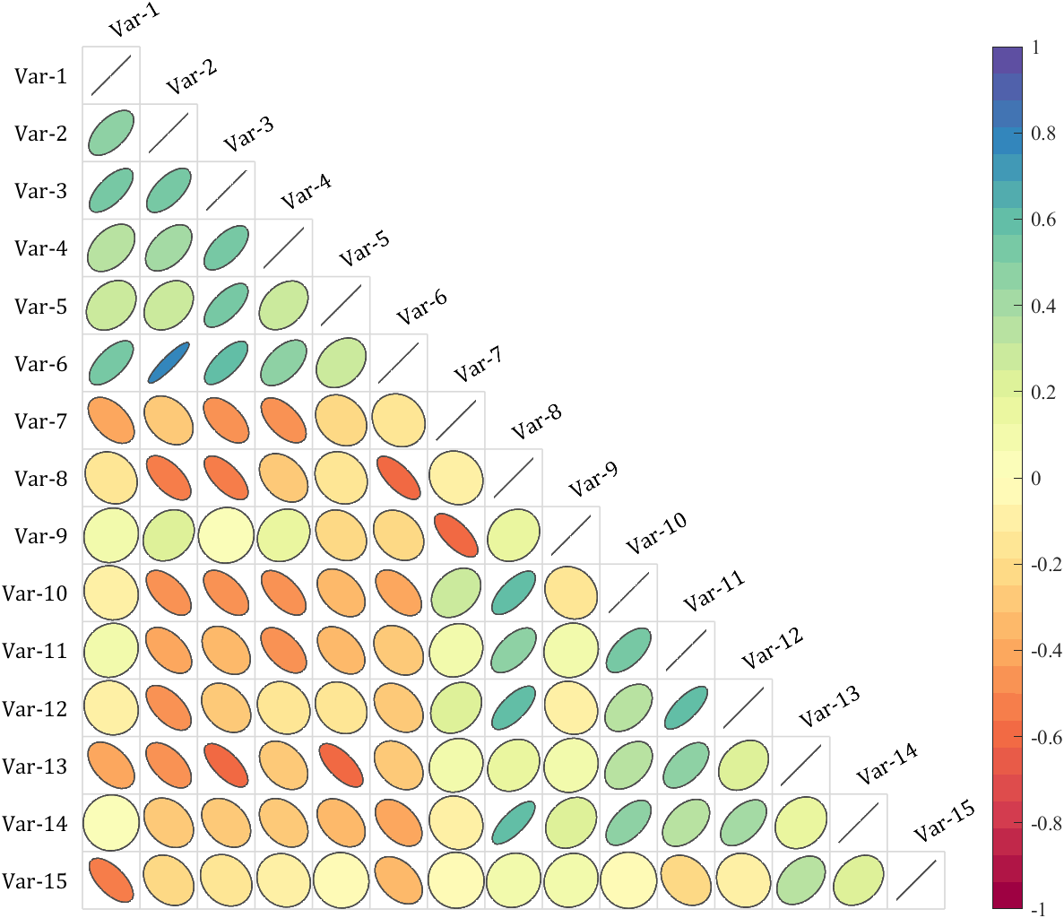
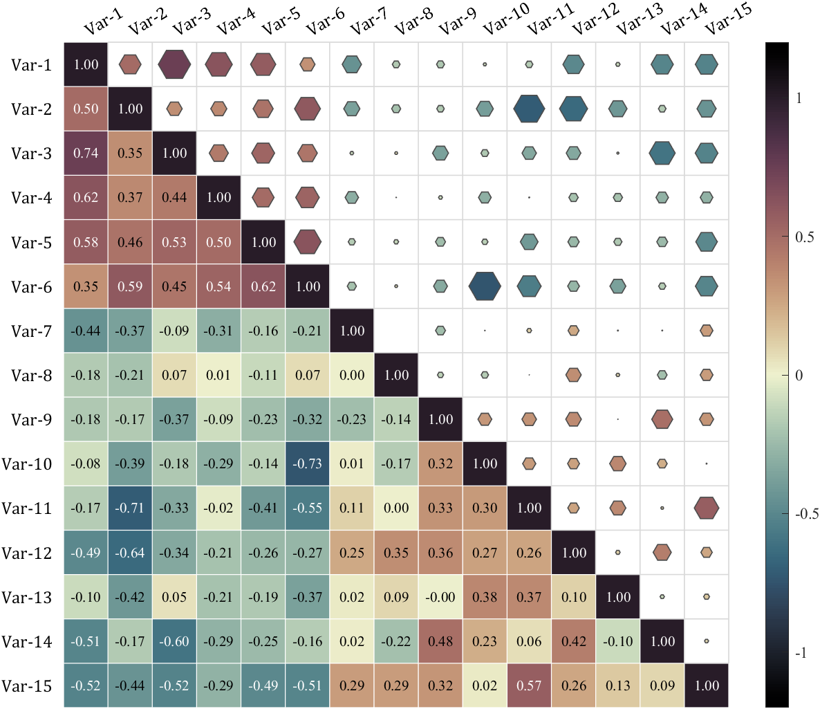
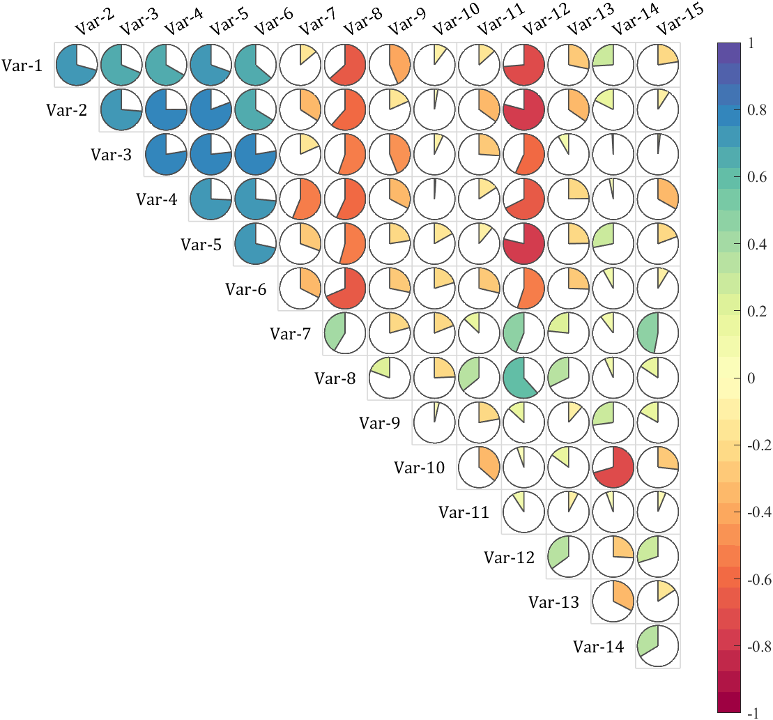
special heatmap
special heatmap
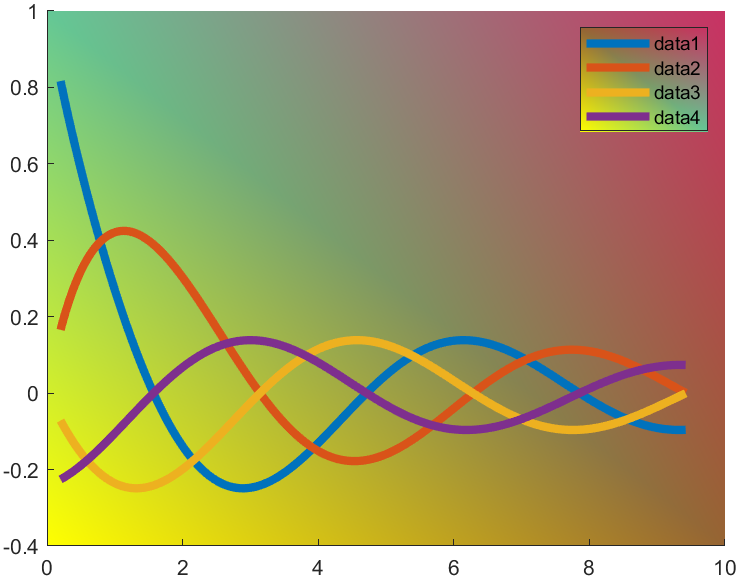
t=0.2:0.01:3*pi;
hold on
plot(t,cos(t)./(1+t),'LineWidth',4)
plot(t,sin(t)./(1+t),'LineWidth',4)
plot(t,cos(t+pi/2)./(1+t+pi/2),'LineWidth',4)
plot(t,cos(t+pi)./(1+t+pi),'LineWidth',4)
ax=gca;
hLegend=legend();
pause(1e-16)
colorData = uint8([255, 150, 200, 100; ...
255, 100, 50, 200; ...
0, 50, 100, 150; ...
102, 150, 200, 50]);
set(ax.Backdrop.Face, 'ColorBinding','interpolated','ColorData',colorData);
set(hLegend.BoxFace,'ColorBinding','interpolated','ColorData',colorData)
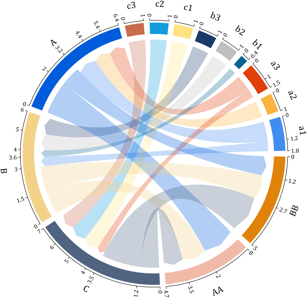
I have written two tools and uploaded fileexchange, which allows us to easily draw chord diagrams:


chord chart 弦图
download:
demo:
dataMat=[2 0 1 2 5 1 2;
3 5 1 4 2 0 1;
4 0 5 5 2 4 3];
dataMat=dataMat+rand(3,7);
dataMat(dataMat<1)=0;
colName={'G1','G2','G3','G4','G5','G6','G7'};
rowName={'S1','S2','S3'};
CC=chordChart(dataMat,'rowName',rowName,'colName',colName);
CC=CC.draw();
CC.setFont('FontSize',17,'FontName','Cambria')
% 显示刻度和数值
% Displays scales and numeric values
CC.tickState('on')
CC.tickLabelState('on')
% 调节标签半径
% Adjustable Label radius
CC.setLabelRadius(1.4);

Digraph chord chart 有向弦图
download:
demo:
dataMat=randi([0,8],[6,6]);
% 添加标签名称
NameList={'CHORD','CHART','MADE','BY','SLANDARER','MATLAB'};
BCC=biChordChart(dataMat,'Label',NameList,'Arrow','on');
BCC=BCC.draw();
% 添加刻度
BCC.tickState('on')
% 修改字体,字号及颜色
BCC.setFont('FontName','Cambria','FontSize',17,'Color',[.2,.2,.2])
BCC.setLabelRadius(1.3);
BCC.tickLabelState('on')
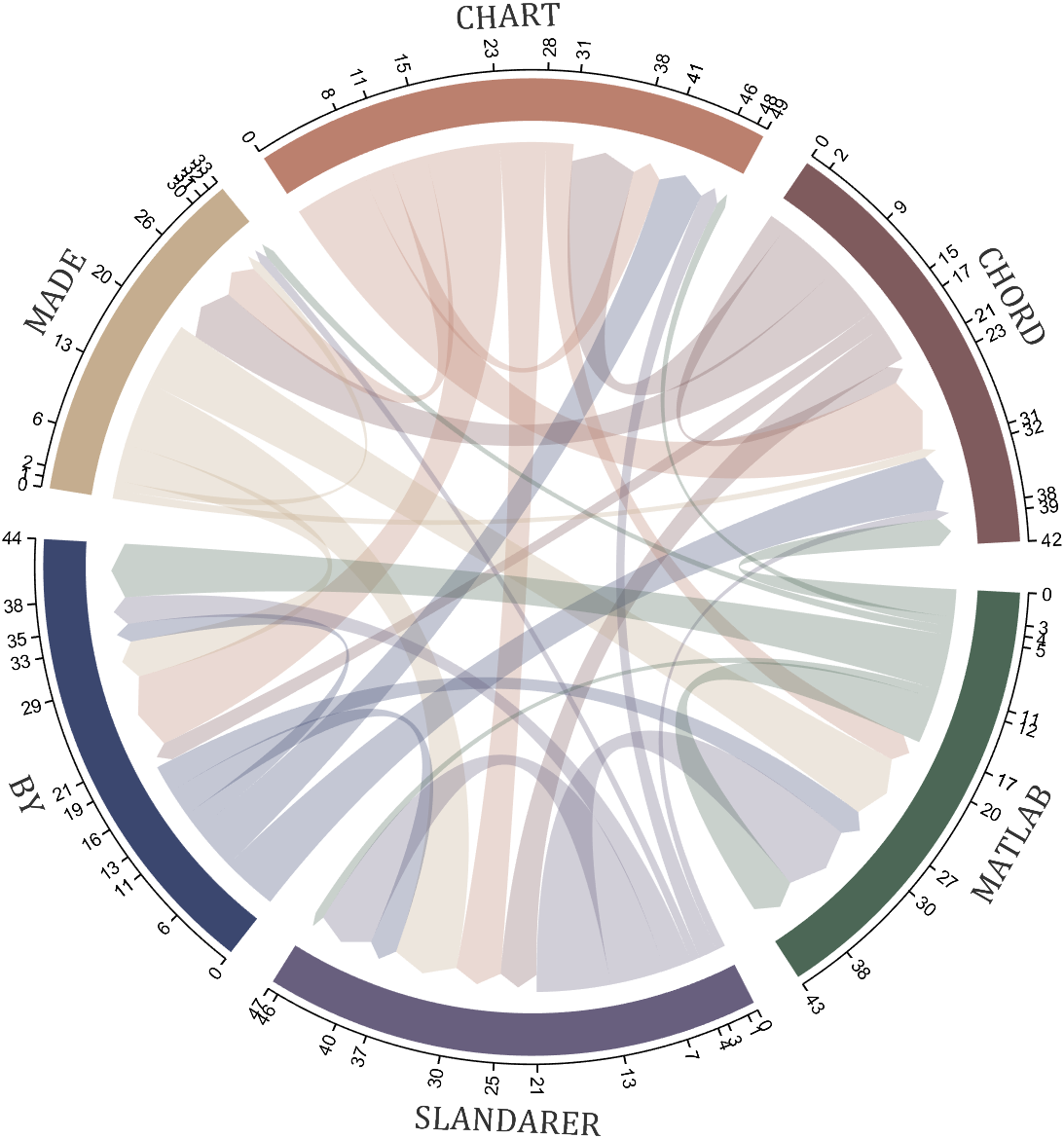
chord chart 弦图
plot beautiful chord chart 好看的弦图绘制
How to create a legend as follows?

Principle Explanation - Graphic Objects
Hidden Properties of Legend are laid as follows
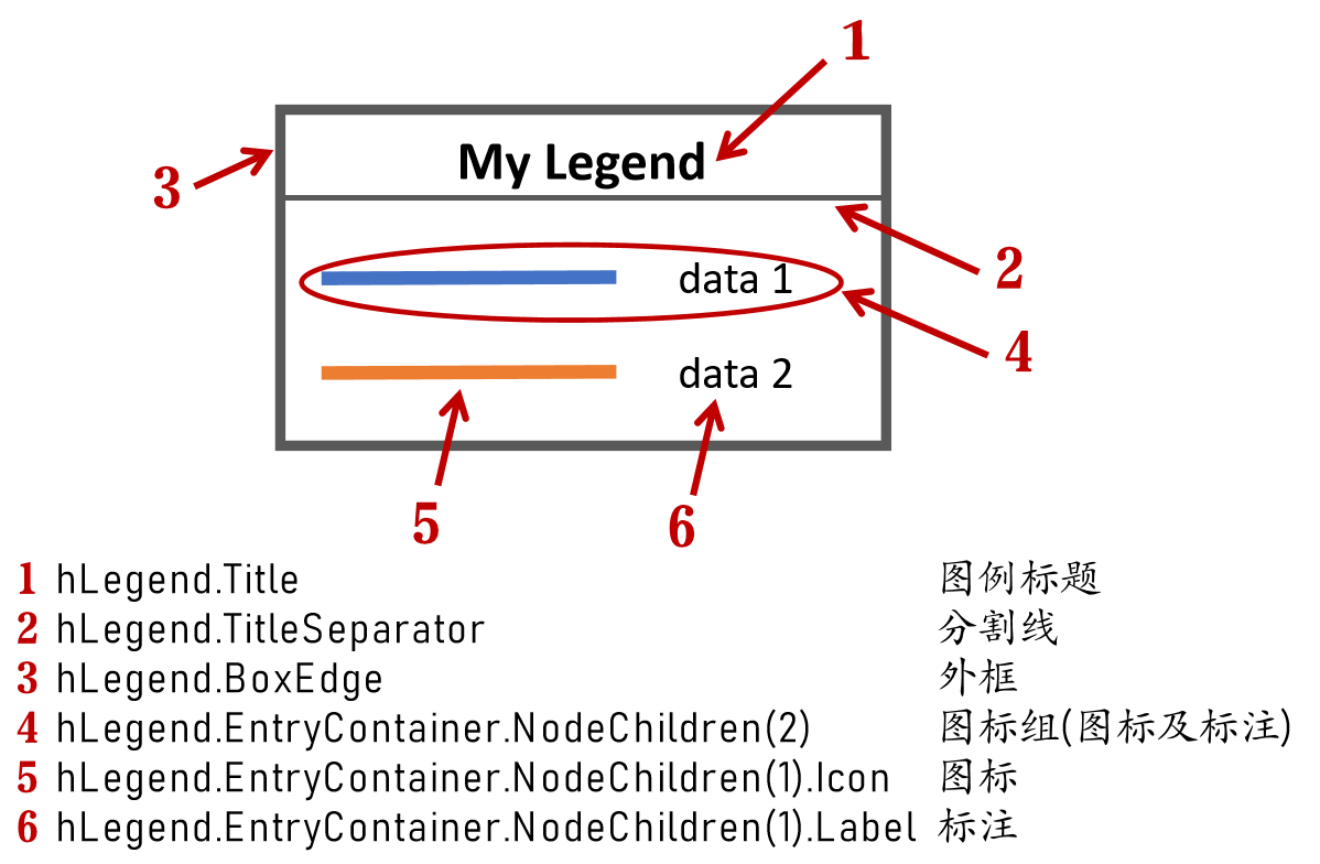
In most cases, legends are drawn using LineLoop and Quadrilateral:
Both of these basic graphic objects are drawn in groups of four points, and the general principle is as follows:

Of course, you can arrange the points in order, or set VertexIndices whitch means the vertex order to obtain the desired quadrilateral shape:

Other objects
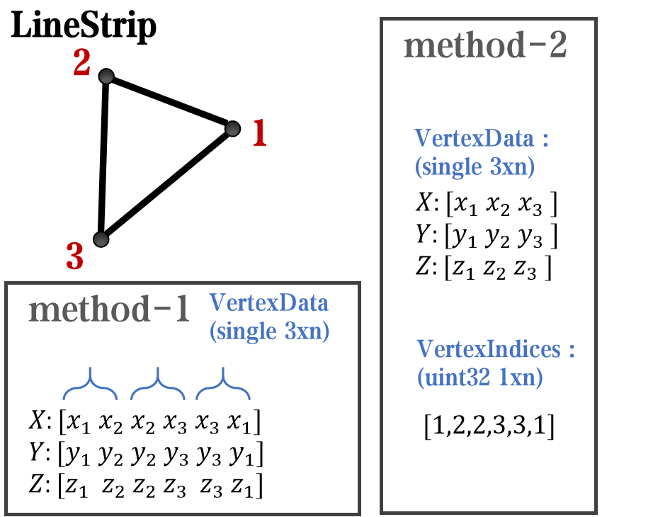
Compared to objects that can only be grouped into four points, we also need to introduce more flexible objects. Firstly, LineStrip, a graphical object that draws lines in groups of two points:
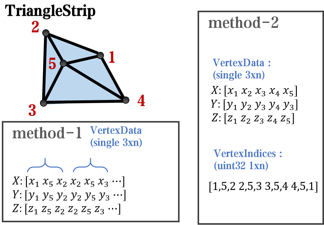
And TriangleStrip is a set of three points that draw objects to fill triangles, for example, complex polygons can be filled with multiple triangles:
Principle Explanation - Create and Replace
Let's talk about how to construct basic graphic objects, which are all constructed using undisclosed and very low-level functions, such as LineStrip, not through:
- LineStrip()
It is built through:
- matlab.graphics.primitive.world.LineStrip()
After building the object, the following properties must be set to make the hidden object visible:
- Layer
- ColorBinding
- ColorData
- VertexData
- PickableParts
The settings of these properties can refer to the original legend to form the object, which will not be elaborated here. You can also refer to the code I wrote.
Afterwards, set the newly constructed object's parent class as the Group parent class of the original component, and then hide the original component
newBoxEdgeHdl.Parent=oriBoxEdgeHdl.Parent;
oriBoxEdgeHdl.Visible='off';
The above is the entire process of component replacement, with two example codes written:
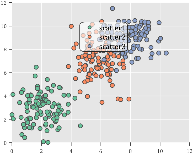
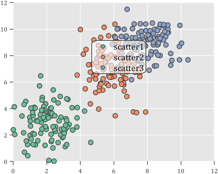
Semi transparent legend
function SPrettyLegend(lgd)
% Semitransparent rounded rectangle legend
% Copyright (c) 2023, Zhaoxu Liu / slandarer
% -------------------------------------------------------------------------
% Zhaoxu Liu / slandarer (2023). pretty legend
% (https://www.mathworks.com/matlabcentral/fileexchange/132128-pretty-legend),
% MATLAB Central File Exchange. 检索来源 2023/7/9.
% =========================================================================
if nargin<1
ax = gca;
lgd = get(ax,'Legend');
end
pause(1e-6)
Ratio = .1;
t1 = linspace(0,pi/2,4); t1 = t1([1,2,2,3,3,4]);
t2 = linspace(pi/2,pi,4); t2 = t2([1,2,2,3,3,4]);
t3 = linspace(pi,3*pi/2,4); t3 = t3([1,2,2,3,3,4]);
t4 = linspace(3*pi/2,2*pi,4); t4 = t4([1,2,2,3,3,4]);
XX = [1,1,1-Ratio+cos(t1).*Ratio,1-Ratio,Ratio,Ratio+cos(t2).*Ratio,...
0,0,Ratio+cos(t3).*Ratio,Ratio,1-Ratio,1-Ratio+cos(t4).*Ratio];
YY = [Ratio,1-Ratio,1-Ratio+sin(t1).*Ratio,1,1,1-Ratio+sin(t2).*Ratio,...
1-Ratio,Ratio,Ratio+sin(t3).*Ratio,0,0,Ratio+sin(t4).*Ratio];
% 圆角边框(border-radius)
oriBoxEdgeHdl = lgd.BoxEdge;
newBoxEdgeHdl = matlab.graphics.primitive.world.LineStrip();
newBoxEdgeHdl.AlignVertexCenters = 'off';
newBoxEdgeHdl.Layer = 'front';
newBoxEdgeHdl.ColorBinding = 'object';
newBoxEdgeHdl.LineWidth = 1;
newBoxEdgeHdl.LineJoin = 'miter';
newBoxEdgeHdl.WideLineRenderingHint = 'software';
newBoxEdgeHdl.ColorData = uint8([38;38;38;0]);
newBoxEdgeHdl.VertexData = single([XX;YY;XX.*0]);
newBoxEdgeHdl.Parent=oriBoxEdgeHdl.Parent;
oriBoxEdgeHdl.Visible='off';
% 半透明圆角背景(Semitransparent rounded background)
oriBoxFaceHdl = lgd.BoxFace;
newBoxFaceHdl = matlab.graphics.primitive.world.TriangleStrip();
Ind = [1:(length(XX)-1);ones(1,length(XX)-1).*(length(XX)+1);2:length(XX)];
Ind = Ind(:).';
newBoxFaceHdl.PickableParts = 'all';
newBoxFaceHdl.Layer = 'back';
newBoxFaceHdl.ColorBinding = 'object';
newBoxFaceHdl.ColorType = 'truecoloralpha';
newBoxFaceHdl.ColorData = uint8(255*[1;1;1;.6]);
newBoxFaceHdl.VertexData = single([XX,.5;YY,.5;XX.*0,0]);
newBoxFaceHdl.VertexIndices = uint32(Ind);
newBoxFaceHdl.Parent = oriBoxFaceHdl.Parent;
oriBoxFaceHdl.Visible = 'off';
end
Usage examples
clc; clear; close all
rng(12)
% 生成随机点(Generate random points)
mu = [2 3; 6 7; 8 9];
S = cat(3,[1 0; 0 2],[1 0; 0 2],[1 0; 0 1]);
r1 = abs(mvnrnd(mu(1,:),S(:,:,1),100));
r2 = abs(mvnrnd(mu(2,:),S(:,:,2),100));
r3 = abs(mvnrnd(mu(3,:),S(:,:,3),100));
% 绘制散点图(Draw scatter chart)
hold on
propCell = {'LineWidth',1.2,'MarkerEdgeColor',[.3,.3,.3],'SizeData',60};
scatter(r1(:,1),r1(:,2),'filled','CData',[0.40 0.76 0.60],propCell{:});
scatter(r2(:,1),r2(:,2),'filled','CData',[0.99 0.55 0.38],propCell{:});
scatter(r3(:,1),r3(:,2),'filled','CData',[0.55 0.63 0.80],propCell{:});
% 增添图例(Draw legend)
lgd = legend('scatter1','scatter2','scatter3');
lgd.Location = 'northwest';
lgd.FontSize = 14;
% 坐标区域基础修饰(Axes basic decoration)
ax=gca; grid on
ax.FontName = 'Cambria';
ax.Color = [0.9,0.9,0.9];
ax.Box = 'off';
ax.TickDir = 'out';
ax.GridColor = [1 1 1];
ax.GridAlpha = 1;
ax.LineWidth = 1;
ax.XColor = [0.2,0.2,0.2];
ax.YColor = [0.2,0.2,0.2];
ax.TickLength = [0.015 0.025];
% 隐藏轴线(Hide XY-Ruler)
pause(1e-6)
ax.XRuler.Axle.LineStyle = 'none';
ax.YRuler.Axle.LineStyle = 'none';
SPrettyLegend(lgd)
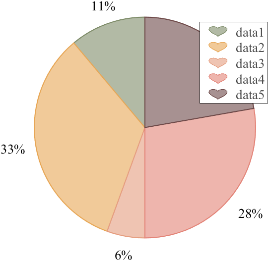
Heart shaped legend (exclusive to pie charts)
function pie2HeartLegend(lgd)
% Heart shaped legend for pie chart
% Copyright (c) 2023, Zhaoxu Liu / slandarer
% -------------------------------------------------------------------------
% Zhaoxu Liu / slandarer (2023). pretty legend
% (https://www.mathworks.com/matlabcentral/fileexchange/132128-pretty-legend),
% MATLAB Central File Exchange. 检索来源 2023/7/9.
% =========================================================================
if nargin<1
ax = gca;
lgd = get(ax,'Legend');
end
pause(1e-6)
% 心形曲线(Heart curve)
x = -1:1/100:1;
y1 = 0.6 * abs(x) .^ 0.5 + ((1 - x .^ 2) / 2) .^ 0.5;
y2 = 0.6 * abs(x) .^ 0.5 - ((1 - x .^ 2) / 2) .^ 0.5;
XX = [x, flip(x),x(1)]./3.4+.5;
YY = ([y1, y2,y1(1)]-.2)./2+.5;
Ind = [1:(length(XX)-1);2:length(XX)];
Ind = Ind(:).';
% 获取图例图标(Get Legend Icon)
lgdEntryChild = lgd.EntryContainer.NodeChildren;
iconSet = arrayfun(@(lgdEntryChild)lgdEntryChild.Icon.Transform.Children.Children,lgdEntryChild,UniformOutput=false);
% 基础边框句柄(Base Border Handle)
newEdgeHdl = matlab.graphics.primitive.world.LineStrip();
newEdgeHdl.AlignVertexCenters = 'off';
newEdgeHdl.Layer = 'front';
newEdgeHdl.ColorBinding = 'object';
newEdgeHdl.LineWidth = .8;
newEdgeHdl.LineJoin = 'miter';
newEdgeHdl.WideLineRenderingHint = 'software';
newEdgeHdl.ColorData = uint8([38;38;38;0]);
newEdgeHdl.VertexData = single([XX;YY;XX.*0]);
newEdgeHdl.VertexIndices = uint32(Ind);
% 基础多边形面句柄(Base Patch Handle)
newFaceHdl = matlab.graphics.primitive.world.TriangleStrip();
Ind = [1:(length(XX)-1);ones(1,length(XX)-1).*(length(XX)+1);2:length(XX)];
Ind = Ind(:).';
newFaceHdl.PickableParts = 'all';
newFaceHdl.Layer = 'middle';
newFaceHdl.ColorBinding = 'object';
newFaceHdl.ColorType = 'truecoloralpha';
newFaceHdl.ColorData = uint8(255*[1;1;1;.6]);
newFaceHdl.VertexData = single([XX,.5;YY,.5;XX.*0,0]);
newFaceHdl.VertexIndices = uint32(Ind);
% 替换图例图标(Replace Legend Icon)
for i = 1:length(iconSet)
oriEdgeHdl = iconSet{i}(1);
tNewEdgeHdl = copy(newEdgeHdl);
tNewEdgeHdl.ColorData = oriEdgeHdl.ColorData;
tNewEdgeHdl.Parent = oriEdgeHdl.Parent;
oriEdgeHdl.Visible = 'off';
oriFaceHdl = iconSet{i}(2);
tNewFaceHdl = copy(newFaceHdl);
tNewFaceHdl.ColorData = oriFaceHdl.ColorData;
tNewFaceHdl.Parent = oriFaceHdl.Parent;
oriFaceHdl.Visible = 'off';
end
end
Usage examples
clc; clear; close all
% 生成随机点(Generate random points)
X = [1 3 0.5 2.5 2];
pieHdl = pie(X);
% 修饰饼状图(Decorate pie chart)
colorList=[0.4941 0.5490 0.4118
0.9059 0.6510 0.3333
0.8980 0.6157 0.4980
0.8902 0.5137 0.4667
0.4275 0.2824 0.2784];
for i = 1:2:length(pieHdl)
pieHdl(i).FaceColor=colorList((i+1)/2,:);
pieHdl(i).EdgeColor=colorList((i+1)/2,:);
pieHdl(i).LineWidth=1;
pieHdl(i).FaceAlpha=.6;
end
for i = 2:2:length(pieHdl)
pieHdl(i).FontSize=13;
pieHdl(i).FontName='Times New Roman';
end
lgd=legend('FontSize',13,'FontName','Times New Roman','TextColor',[1,1,1].*.3);
pie2HeartLegend(lgd)
I am confused, is the matlab answer better or Julia’s?
Hello and a warm welcome to all! We're thrilled to have you visit our community. MATLAB Central is a place for learning, sharing, and connecting with others who share your passion for MATLAB and Simulink. To ensure you have the best experience, here are some tips to get you started:
- Read the Community Guidelines: Understanding our community standards is crucial. Please take a moment to familiarize yourself with them. Keep in mind that posts not adhering to these guidelines may be flagged by moderators or other community members.
- Ask Technical Questions at MATLAB Answers: If you have questions related to MathWorks products, head over to MATLAB Answers (new question form - Ask the community). It's the go-to spot for technical inquiries, with responses often provided within an hour, depending on the complexity of the question and volunteer availability. To increase your chances of a speedy reply, check out our tips on how to craft a good question (link to post on asking good questions).
- Choosing the Right Channel: We offer a variety of discussion channels tailored to different contexts. Select the one that best fits your post. If you're unsure, the General channel is always a safe bet. If you feel there's a need for a new channel, we encourage you to suggest it in the Ideas channel.
- Reporting Issues: If you encounter posts that violate our guidelines, please use the 🚩Flag/Report feature (found in the 3-dot menu) to bring them to our attention.
- Quality Control: We strive to maintain a high standard of discussion. Accounts that post spam or too much nonsense may be subject to moderation, which can include temporary suspensions or permanent bans.
- Share Your Ideas: Your feedback is invaluable. If you have suggestions on how we can improve the community or MathWorks products, the Ideas channel is the perfect place to voice your thoughts.
Enjoy yourself and have fun! We're committed to fostering a supportive and educational environment. Dive into discussions, share your expertise, and grow your knowledge. We're excited to see what you'll contribute to the community!
I recently discovered a 2-minute video that introduces MatGPT, and I believe it's a resource worth sharing. The creator highlights MatGPT's impressive capabilities by demonstrating how it tackles the classic Travelling Salesman Problem.
With more than 13,000 downloads on File Exchange, MatGPT is gaining traction among users. I strongly recommend taking it for a spin to experience its potential firsthand.
I found this list on Book Authority about the top MATLAB books: https://bookauthority.org/books/best-matlab-books
My favorite book is Accelerating MATLAB Performance - 1001 tips to speed up MATLAB programs. I always pick something up from the book that helps me out.
Have you ever used Live Tasks in MATLAB? MathWorks development team would like to get some feedback on your experience – what did you like and not like. Especially, if you know about it but don’t use it frequently, we would like to understand why?
Please tell us what you think by submitting your response to this form https://forms.office.com/r/ui1EGqAFDx
how accurate are the answers of the AI Playground regarding information that are not specifiyed in the documentation?
A key aspect to masting MATLAB Graphics is getting a hang of the MATLAB Graphics Object Hierarchy which is essentially the structure of MATLAB figures that is used in the rendering pipeline. The base object is the Graphics Root (see groot) which contains the Figure. The Figure contains Axes or other containers such as a Tiled Chart Layout (see tiledlayout). Then these Axes can contain graphics primatives (the objects that contain data and get rendered) such as Lines or Patches.
Every graphics object has two important properties, the "Parent" and "Children" properties which can be used to access other objects in the tree. This can be very useful when trying to customize a pre-built chart (such as adding grid lines to both axes in an eye diagram chart) or when trying to access the axes of a non-current figure via a primative (so "gca" doesn't help out).
One last Tip and Trick with this is that you can declare graphics primatives without putting them on or creating an Axes by setting the first input argument to "gobjects(0)" which is an empty array of placeholder graphics objects. Then, when you have an Axes to plot the primitive on and are ready to render it, you can set the "Parent" of the object to your new Axes.
For Example:
l = line(gobjects(0), 1:10, 1:10);
...
...
...
l.Parent = gca;
Practicing navigating and exploring this tree will help propel your understanding of plotting in MATLAB.
We're thrilled to announce the roll-out of some new features that are going to supercharge your Playground experience! Here's what's new:
Copy/Download code from the script area
You can now effortlessly Copy/Download code from the script area with just a single click. Copy code or Download your script directly as .m files and keep your work organized and portable.We hope this will allow you to effortlessly transfer your work from Playground to MATLAB Desktop/Online.
Run Code directly from the Chat panel
Execute code snippets from the chat section with a single click. This new affordance means saving a step since you no longer have to insert code and then hit run from the toolstrip to execute instead just hit run in the chat panel to see the output immediately in the script area
Enhanced visual Experience
Customize your Playground workspace by expanding or collapsing the chat and script sections. Focus on what matters most to you, whether it's AI chat or working on your script.
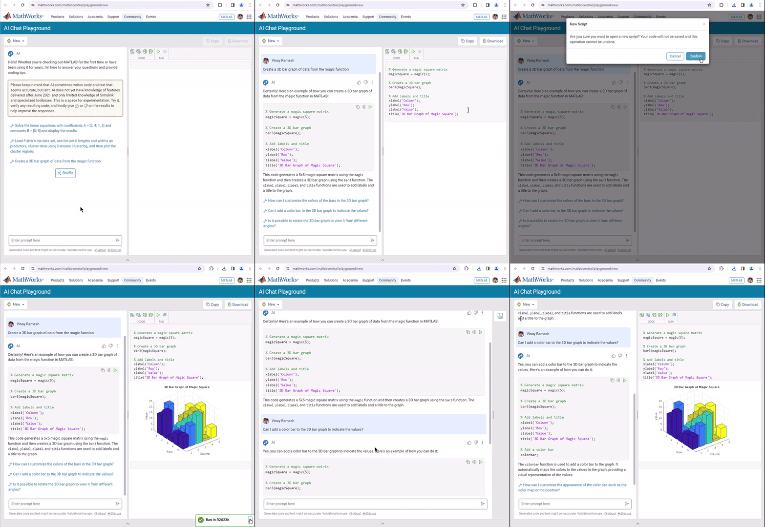
We hope you will love these updates. Try them out and let us know your feedback.
MathWorks just released three new courses on Coursera liseted below. If you work with image or video data and are wanting to incorporate deep learning techniques into your workflow, this is a great opporutnity. The course creators monitor the discussion forums, so you can ask questions and get feedback on your work. Below are links to the three courses and a quick description of a project you'll complete in each.
- Introduction to Computer Vision for Deep Learning. You'll train a classifier to classify images of people signing the American Sign Language alphabet.
- Deep Learning for Object Detection. Move from just classification to finding object locations. You'll train a model to find different types of parking available on the MathWorks campus.
- Advanced Deep Learning Techniques for Computer Vision. You'll train anomaly detection models for medical images and use AI-assisted labeling auto label images.


