主要内容
Results for
isempty( [ ] )
10%
isempty( { } )
13%
isempty( '' ) % 2 single quotes
13%
isempty( "" ) % 2 double quotes
24%
c = categorical( [ ] ); isempty(c)
18%
s = struct("a", [ ] ); isempty(s.a)
22%
1324 个投票
Looking for 10 candidates for a closed beta on new MATLAB live script features.
Do you use live scripts regularly in MATLAB? Do you collaborate with others using live scripts?
MathWorks is looking for 10 candidates for a closed beta on new features for live scripts. Help us develop exciting new features with your feedback.
If you are selected, you will receive an email invitation to sign an NDA
I will post here when the quota is filled

The image was created with DALL-E 3.
Hello, brilliant minds of our engineering community!
We hope this message finds you in the midst of an exciting project or, perhaps, deep in the realms of a challenging problem, because we've got some groundbreaking news that might just make your day a whole lot more interesting.

🎉 Introducing PreAnswer AI - The Future of Community Support! 🎉
Have you ever found yourself pondering over a complex problem, wishing for an answer to magically appear before you even finish formulating the question? Well, wish no more! The MathWorks team, in collaboration with the most imaginative minds from the realms of science fiction, is thrilled to announce the launch of PreAnswer AI, an unprecedented feature set to revolutionize the way we interact within our MATLAB and Simulink community.
What is PreAnswer AI?
PreAnswer AI is our latest AI-driven initiative designed to answer your questions before you even ask them. Yes, you read that right! Through a combination of predictive analytics, machine learning, and a pinch of engineering wizardry, PreAnswer AI anticipates the challenges you're facing and provides you with solutions, insights, and code snippets in real-time.
How Does It Work?
- Presentiment Algorithms: By simply logging into MATLAB Central, our AI begins to analyze your recent coding patterns, activity, and even the intensity of your keyboard strokes to understand your current state of mind.
- Predictive Insights: Using a complex algorithm, affectionately dubbed "The Oracle", PreAnswer AI predicts the questions you're likely to ask and compiles comprehensive answers from our vast database of resources.
- Efficiency and Speed: Imagine the time saved when the answers to your questions are already waiting for you. PreAnswer AI ensures you spend more time innovating and less time searching for solutions.
We are on the cusp of deploying PreAnswer AI in a beta phase and are eager for you to be among the first to experience its benefits. Your feedback will be invaluable as we refine this feature to better suit our community's needs.
---------------------------------------------------------------
Spoiler, it's April 1st if you hadn't noticed. While we might not (yet) have the technology to read minds or predict the future, we do have an incredible community filled with knowledgeable, supportive members ready to tackle any question you throw their way.
Let's continue to collaborate, innovate, and solve complex problems together, proving that while AI can do many things, the power of a united community of brilliant minds is truly unmatched.
Thank you for being such a fantastic part of our community. Here's to many more questions, answers, and shared laughs along the way.
Happy April Fools' Day!
The line integral  , where C is the boundary of the square
  oriented counterclockwise, can be evaluated in two ways:
 , where C is the boundary of the square
 Using the definition of the line integral:
% Initialize the integral sum
integral_sum = 0;
% Segment C1: x = -1, y goes from -1 to 1
y = linspace(-1, 1);
x = -1 * ones(size(y));
dy = diff(y);
integral_sum = integral_sum + sum(-x(1:end-1) .* dy);
% Segment C2: y = 1, x goes from -1 to 1
x = linspace(-1, 1);
y = ones(size(x));
dx = diff(x);
integral_sum = integral_sum + sum(y(1:end-1).^2 .* dx);
% Segment C3: x = 1, y goes from 1 to -1
y = linspace(1, -1);
x = ones(size(y));
dy = diff(y);
integral_sum = integral_sum + sum(-x(1:end-1) .* dy);
% Segment C4: y = -1, x goes from 1 to -1
x = linspace(1, -1);
y = -1 * ones(size(x));
dx = diff(x);
integral_sum = integral_sum + sum(y(1:end-1).^2 .* dx);
disp(['Direct Method Integral: ', num2str(integral_sum)]);
Plotting the square path
% Define the square's vertices
vertices = [-1 -1; -1 1; 1 1; 1 -1; -1 -1];
% Plot the square
figure;
plot(vertices(:,1), vertices(:,2), '-o');
title('Square Path for Line Integral');
xlabel('x');
ylabel('y');
grid on;
axis equal;
% Add arrows to indicate the path direction (counterclockwise)
hold on;
for i = 1:size(vertices,1)-1
% Calculate direction
dx = vertices(i+1,1) - vertices(i,1);
dy = vertices(i+1,2) - vertices(i,2);
% Reduce the length of the arrow for better visibility
scale = 0.2;
dx = scale * dx;
dy = scale * dy;
% Calculate the start point of the arrow
startx = vertices(i,1) + (1 - scale) * dx;
starty = vertices(i,2) + (1 - scale) * dy;
% Plot the arrow
quiver(startx, starty, dx, dy, 'MaxHeadSize', 0.5, 'Color', 'r', 'AutoScale', 'off');
end
hold off;

Apply Green's Theorem for the line integral
% Define the partial derivatives of P and Q
f = @(x, y) -1 - 2*y; % derivative of -x with respect to x is -1, and derivative of y^2 with respect to y is 2y
% Compute the double integral over the square [-1,1]x[-1,1]
integral_value = integral2(f, -1, 1, 1, -1);
disp(['Green''s Theorem Integral: ', num2str(integral_value)]);
Plotting the vector field related to Green’s theorem
% Define the grid for the vector field
[x, y] = meshgrid(linspace(-2, 2, 20), linspace(-2 ,2, 20));
% Define the vector field components
P = y.^2; % y^2 component
Q = -x; % -x component
% Plot the vector field
figure;
quiver(x, y, P, Q, 'b');
hold on; % Hold on to plot the square on the same figure
% Define the square's vertices
vertices = [-1 -1; -1 1; 1 1; 1 -1; -1 -1];
% Plot the square path
plot(vertices(:,1), vertices(:,2), '-o', 'Color', 'k'); % 'k' for black color
title('Vector Field (P = y^2, Q = -x) with Square Path');
xlabel('x');
ylabel('y');
axis equal;
% Add arrows to indicate the path direction (counterclockwise)
for i = 1:size(vertices,1)-1
% Calculate direction
dx = vertices(i+1,1) - vertices(i,1);
dy = vertices(i+1,2) - vertices(i,2);
% Reduce the length of the arrow for better visibility
scale = 0.2;
dx = scale * dx;
dy = scale * dy;
% Calculate the start point of the arrow
startx = vertices(i,1) + (1 - scale) * dx;
starty = vertices(i,2) + (1 - scale) * dy;
% Plot the arrow
quiver(startx, starty, dx, dy, 'MaxHeadSize', 0.5, 'Color', 'r', 'AutoScale', 'off');
end
hold off;

To solve a surface integral for example the over the sphere
  easily in MATLAB, you can leverage the symbolic toolbox for a direct and clear solution. Here is a tip to simplify the process:
 over the sphere
 - Use Symbolic Variables and Functions: Define your variables symbolically, including the parameters of your spherical coordinates θ and ϕ and the radius r . This allows MATLAB to handle the expressions symbolically, making it easier to manipulate and integrate them.
- Express in Spherical Coordinates Directly: Since you already know the sphere's equation and the relationship in spherical coordinates, define x, y, and z in terms of r , θ and ϕ directly.
- Perform Symbolic Integration: Use MATLAB's `int` function to integrate symbolically. Since the sphere and the function
 are symmetric, you can exploit these symmetries to simplify the calculation.
Here’s how you can apply this tip in MATLAB code:
% Include the symbolic math toolbox
syms theta phi
% Define the limits for theta and phi
theta_limits = [0, pi];
phi_limits = [0, 2*pi];
% Define the integrand function symbolically
integrand = 16 * sin(theta)^3 * cos(phi)^2;
% Perform the symbolic integral for the surface integral
surface_integral = int(int(integrand, theta, theta_limits(1), theta_limits(2)), phi, phi_limits(1), phi_limits(2));
% Display the result of the surface integral symbolically
disp(['The surface integral of x^2 over the sphere is ', char(surface_integral)]);
% Number of points for plotting
num_points = 100;
% Define theta and phi for the sphere's surface
[theta_mesh, phi_mesh] = meshgrid(linspace(double(theta_limits(1)), double(theta_limits(2)), num_points), ...
linspace(double(phi_limits(1)), double(phi_limits(2)), num_points));
% Spherical to Cartesian conversion for plotting
r = 2; % radius of the sphere
x = r * sin(theta_mesh) .* cos(phi_mesh);
y = r * sin(theta_mesh) .* sin(phi_mesh);
z = r * cos(theta_mesh);
% Plot the sphere
figure;
surf(x, y, z, 'FaceColor', 'interp', 'EdgeColor', 'none');
colormap('jet'); % Color scheme
shading interp; % Smooth shading
camlight headlight; % Add headlight-type lighting
lighting gouraud; % Use Gouraud shading for smooth color transitions
title('Sphere: x^2 + y^2 + z^2 = 4');
xlabel('x-axis');
ylabel('y-axis');
zlabel('z-axis');
colorbar; % Add color bar to indicate height values
axis square; % Maintain aspect ratio to be square
view([-30, 20]); % Set a nice viewing angle

I am often talking to new MATLAB users. I have put together one script. If you know how this script works, why, and what each line means, you will be well on your way on your MATLAB learning journey.
% Clear existing variables and close figures
clear;
close all;
% Print to the Command Window
disp('Hello, welcome to MATLAB!');
% Create a simple vector and matrix
vector = [1, 2, 3, 4, 5];
matrix = [1, 2, 3; 4, 5, 6; 7, 8, 9];
% Display the created vector and matrix
disp('Created vector:');
disp(vector);
disp('Created matrix:');
disp(matrix);
% Perform element-wise multiplication
result = vector .* 2;
% Display the result of the operation
disp('Result of element-wise multiplication of the vector by 2:');
disp(result);
% Create plot
x = 0:0.1:2*pi; % Generate values from 0 to 2*pi
y = sin(x); % Calculate the sine of these values
% Plotting
figure; % Create a new figure window
plot(x, y); % Plot x vs. y
title('Simple Plot of sin(x)'); % Give the plot a title
xlabel('x'); % Label the x-axis
ylabel('sin(x)'); % Label the y-axis
grid on; % Turn on the grid
disp('This is the end of the script. Explore MATLAB further to learn more!');
More than 500,000 people have subscribed to the MATLAB channel. MathWorks would like to thank everyone who has taken the time to watch one of our videos, leave us a comment, or share our videos with others. Together we’re accelerating the pace of engineering and science.
Although, I think I will only get to see a partial eclipse (April 8th!) from where I am at in the U.S. I will always have MATLAB to make my own solar eclipse. Just as good as the real thing.
Code (found on the @MATLAB instagram)
a=716;
v=255;
X=linspace(-10,10,a);
[~,r]=cart2pol(X,X');
colormap(gray.*[1 .78 .3]);
[t,g]=cart2pol(X+2.6,X'+1.4);
image(rescale(-1*(2*sin(t*10)+60*g.^.2),0,v))
hold on
h=exp(-(r-3)).*abs(ifft2(r.^-1.8.*cos(7*rand(a))));
h(r<3)=0;
image(v*ones(a),'AlphaData',rescale(h,0,1))
camva(3.8)

One of the privileges of working at MathWorks is that I get to hang out with some really amazing people. Steve Eddins, of ‘Steve on Image Processing’ fame is one of those people. He recently announced his retirement and before his final day, I got the chance to interview him. See what he had to say over at The MATLAB Blog The Steve Eddins Interview: 30 years of MathWorking
Before we begin, you will need to make sure you have 'sir_age_model.m' installed. Once you've downloaded this folder into your working directory, which can be located at your current folder. If you can see this file in your current folder, then it's safe to use it. If you choose to use MATLAB online or MATLAB Mobile, you may upload this to your MATLAB Drive.
This is the code for the SIR model stratified into 2 age groups (children and adults). For a detailed explanation of how to derive the force of infection by age group.
% Main script to run the SIR model simulation
% Initial state values
initial_state_values = [200000; 1; 0; 800000; 0; 0]; % [S1; I1; R1; S2; I2; R2]
% Parameters
parameters = [0.05; 7; 6; 1; 10; 1/5]; % [b; c_11; c_12; c_21; c_22; gamma]
% Time span for the simulation (3 months, with daily steps)
tspan = [0 90];
% Solve the ODE
[t, y] = ode45(@(t, y) sir_age_model(t, y, parameters), tspan, initial_state_values);
% Plotting the results
plot(t, y);
xlabel('Time (days)');
ylabel('Number of people');
legend('S1', 'I1', 'R1', 'S2', 'I2', 'R2');
title('SIR Model with Age Structure');

What was the cumulative incidence of infection during this epidemic? What proportion of those infections occurred in children?
In the SIR model, the cumulative incidence of infection is simply the decline in susceptibility.
% Assuming 'y' contains the simulation results from the ode45 function
% and 't' contains the time points
% Total cumulative incidence
total_cumulative_incidence = (y(1,1) - y(end,1)) + (y(1,4) - y(end,4));
fprintf('Total cumulative incidence: %f\n', total_cumulative_incidence);
% Cumulative incidence in children
cumulative_incidence_children = (y(1,1) - y(end,1));
% Proportion of infections in children
proportion_infections_children = cumulative_incidence_children / total_cumulative_incidence;
fprintf('Proportion of infections in children: %f\n', proportion_infections_children);
927,447 people became infected during this epidemic, 20.5% of which were children.
Which age group was most affected by the epidemic?
To answer this, we can calculate the proportion of children and adults that became infected.
% Assuming 'y' contains the simulation results from the ode45 function
% and 't' contains the time points
% Proportion of children that became infected
initial_children = 200000; % initial number of susceptible children
final_susceptible_children = y(end,1); % final number of susceptible children
proportion_infected_children = (initial_children - final_susceptible_children) / initial_children;
fprintf('Proportion of children that became infected: %f\n', proportion_infected_children);
% Proportion of adults that became infected
initial_adults = 800000; % initial number of susceptible adults
final_susceptible_adults = y(end,4); % final number of susceptible adults
proportion_infected_adults = (initial_adults - final_susceptible_adults) / initial_adults;
fprintf('Proportion of adults that became infected: %f\n', proportion_infected_adults);
Throughout this epidemic, 95% of all children and 92% of all adults were infected. Children were therefore slightly more affected in proportion to their population size, even though the majority of infections occurred in adults.
Are you going to be in the path of totality? How can you predict, track, and simulate the solar eclipse using MATLAB?
Hey MATLAB Community! 🌟
March has been bustling with activity on MATLAB Central, bringing forth a treasure trove of insights, innovations, and fun. Whether you're delving into the intricacies of spline conversions or seeking inspiration from Pi Day celebrations, there's something for everyone.
Here’s a roundup of the top posts from the past few weeks that you won't want to miss:
Interesting questions
Dive into the technicalities of converting spline forms with a focus on calculating coefficients. A must-read for anyone dealing with spline representations.
Explore the challenges and solutions in tuning autopilot gains within a non-linear model of a business jet aircraft.
Popular discussions
Celebrate Pi Day with cool MATLAB implementations and code. A delightful read filled with π-inspired creativity.
Get a glimpse of fun with MATLAB through an engaging visual shared by Athanasios. A light-hearted thread that showcases the fun side of mathematics.
From File Exchange
Unlock the secrets of global climate data with MATLAB. This thread offers tools and insights for analyzing precipitation variability.
Interact with a numerical puddle in real-time and explore the dynamics of disturbances. A fascinating exploration of fluid dynamics simulation.
From the Blogs
Revisit Pi Day with Jiro's picks of the coolest π visualizations. A post that combines art, math, and the joy of exploration.
Discover the synergy between MATLAB and Visual Studio Code, enhanced by GitHub Copilot support. A game-changer for MATLAB developers.
These threads are just the tip of the iceberg. Each post is a gateway to new knowledge, ideas, and community connections. Dive in, explore, and don't forget to contribute your insights and questions. Together, we make MATLAB Central a vibrant hub of innovation and support.
Happy Coding!
The latest release is pretty much upon us. Official annoucements will be coming soon and the eagle-eyed among you will have started to notice some things shifting around on the MathWorks website as we ready for this.
The pre-release has been available for a while. Maybe you've played with it? I have...I've even been quietly using it to write some of my latest blog posts...and I have several queued up for publication after MathWorks officially drops the release.
At the time of writing, this page points to the pre-release highlights. Prerelease Release Highlights - MATLAB & Simulink (mathworks.com)
What excites you about this release? why?
sort(v)
8%
unique(v)
16%
union(v, [ ])
17%
intersect(v, v)
14%
setdiff(v, [ ])
12%
All return sorted output
33%
1193 个投票
The stationary solutions of the Klein-Gordon equation refer to solutions that are time-independent, meaning they remain constant over time. For the non-linear Klein-Gordon equation you are discussing:

Stationary solutions arise when the time derivative term,  , is zero, meaning the motion of the system does not change over time. This leads to a static differential equation:
 , is zero, meaning the motion of the system does not change over time. This leads to a static differential equation:
This equation describes how particles in the lattice interact with each other and how non-linearity affects the steady state of the system.
The solutions to this equation correspond to the various possible stable equilibrium states of the system, where each represents different static distribution patterns of displacements  . The specific form of these stationary solutions depends on the system parameters, such as κ , ω, and β , as well as the initial and boundary conditions of the problem.
To find these solutions in a more specific form, one might need to solve the equation using analytical or numerical methods, considering the different cases that could arise in such a non-linear system.
By interpreting the equation in this way, we can relate the dynamics described by the discrete Klein - Gordon equation to the behavior of DNA molecules within a biological system . This analogy allows us to understand the behavior of DNA in terms of concepts from physics and mathematical modeling .
% Parameters
numBases = 100; % Number of spatial points
omegaD = 0.2; % Common parameter for the equation
% Preallocate the array for the function handles
equations = cell(numBases, 1);
% Initial guess for the solution
initialGuess = 0.01 * ones(numBases, 1);
% Parameter sets for kappa and beta
paramSets = [0.1, 0.05; 0.5, 0.05; 0.1, 0.2];
% Prepare figure for subplot
figure;
set(gcf, 'Position', [100, 100, 1200, 400]); % Set figure size
% Newton-Raphson method parameters
maxIterations = 1000;
tolerance = 1e-10;
% Set options for fsolve to use the 'levenberg-marquardt' algorithm
options = optimoptions('fsolve', 'Algorithm', 'levenberg-marquardt', 'MaxIterations', maxIterations, 'FunctionTolerance', tolerance);
for i = 1:size(paramSets, 1)
kappa = paramSets(i, 1);
beta = paramSets(i, 2);
% Define the equations using a function
for n = 2:numBases-1
equations{n} = @(x) -kappa * (x(n+1) - 2 * x(n) + x(n-1)) - omegaD^2 * (x(n) - beta * x(n)^3);
end
% Boundary conditions with specified fixed values
someFixedValue1 = 10; % Replace with actual value if needed
someFixedValue2 = 10; % Replace with actual value if needed
equations{1} = @(x) x(1) - someFixedValue1;
equations{numBases} = @(x) x(numBases) - someFixedValue2;
% Combine all equations into a single function
F = @(x) cell2mat(cellfun(@(f) f(x), equations, 'UniformOutput', false));
% Solve the system of equations using fsolve with the specified options
x_solution = fsolve(F, initialGuess, options);
norm(F(x_solution))
% Plot the solution in a subplot
subplot(1, 3, i);
plot(x_solution, 'o-', 'LineWidth', 2);
grid on;
xlabel('n', 'FontSize', 12);
ylabel('x[n]', 'FontSize', 12);
title(sprintf('\\kappa = %.2f, \\beta = %.2f', kappa, beta), 'FontSize', 14);
end
% Improve overall aesthetics
sgtitle('Stationary States for Different \kappa and \beta Values', 'FontSize', 16); % Super title for the figure
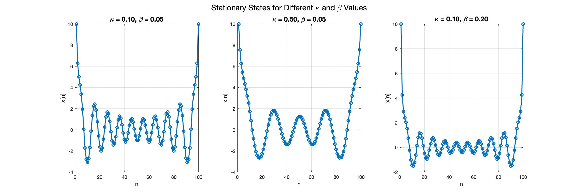
In the second plot, the elasticity constant κis increased to 0.5, representing a system with greater stiffness . This parameter influences how resistant the system is to deformation, implying that a higher κ makes the system more resilient to changes . By increasing κ, we are essentially tightening the interactions between adjacent units in the model, which could represent, for instance, stronger bonding forces in a physical or biological system .
In the third plot the nonlinearity coefficient β is increased to 0.2 . This adjustment enhances the nonlinear interactions within the system, which can lead to more complex dynamic behaviors, especially in systems exhibiting bifurcations or chaos under certain conditions .
The following expression 

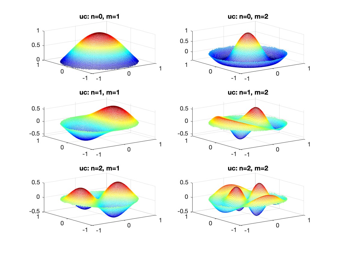
gives the solution for the Helmholtz problem. On the circular disc with center 0 and radius a. For  the plot in 3-dimensional graphics of the solutions on Matlab for
  and then calculate some eigenfunctions with the following expression.

It could be better to separate functions with  and
and  as follows
diska = 1; % Radius of the disk
mmax = 2; % Maximum value of m
nmax = 2; % Maximum value of n
% Function to find the k-th zero of the n-th Bessel function
% This function uses a more accurate method for initial guess
besselzero = @(n, k) fzero(@(x) besselj(n, x), [(k-(n==0))*pi, (k+1-(n==0))*pi]);
% Define the eigenvalue k[m, n] based on the zeros of the Bessel function
k = @(m, n) besselzero(n, m);
% Define the functions uc and us using Bessel functions
% These functions represent the radial part of the solution
uc = @(r, t, m, n) cos(n * t) .* besselj(n, k(m, n) * r);
us = @(r, t, m, n) sin(n * t) .* besselj(n, k(m, n) * r);
% Generate data for demonstration
data = zeros(5, 3);
for m = 1:5
for n = 0:2
data(m, n+1) = k(m, n); % Storing the eigenvalues
end
end
% Display the data
disp(data);
% Plotting all in one figure
figure;
plotIndex = 1;
for n = 0:nmax
for m = 1:mmax
subplot(nmax + 1, mmax, plotIndex);
[X, Y] = meshgrid(linspace(-diska, diska, 100), linspace(-diska, diska, 100));
R = sqrt(X.^2 + Y.^2);
T = atan2(Y, X);
Z = uc(R, T, m, n); % Using uc for plotting
% Ensure the plot is only within the disk
Z(R > diska) = NaN;
mesh(X, Y, Z);
title(sprintf('uc: n=%d, m=%d', n, m));
colormap('jet');
plotIndex = plotIndex + 1;
end
end
First, I felt that the three answers provided by a user in this thread might have been generated by AI. How do you think?
Second, I found that "Responsible usage of generative AI tools, such as ChatGPT, is allowed in MATLAB Answers."
If the answers are indeed AI generated, then the user didn't do "clearly indicating when AI generated content is incorporated".
That leads to my question that how do we enforce the guideline.
I am not against using AI for answers but in this case, I felt the answering text is mentioning all the relevant words but missing the point. For novice users who are seeking answers, this would be misleading and waste of time.
Happy Pi Day!
3.14 π Day has arrived, and this post provides some very cool pi implementations and complete MATLAB code.
Firstly, in order to obtain the first n decimal places of pi, we need to write the following code (to prevent inaccuracies, we need to take a few more tails and perform another operation of taking the first n decimal places when needed):
function Pi=getPi(n)
if nargin<1,n=3;end
Pi=char(vpa(sym(pi),n+10));
Pi=abs(Pi)-48;
Pi=Pi(3:n+2);
end
With this function to obtain the decimal places of pi, our visualization journey has begun~Step by step, from simple to complex~(Please try to use newer versions of MATLAB to run, at least R17b)
1 Pie chart
Just calculate the proportion of each digit to the first 1500 decimal places:
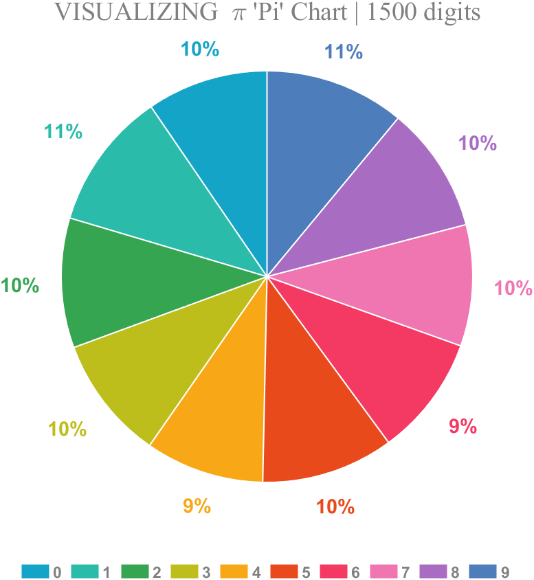
% 获取pi前1500位小数
Pi=getPi(1500);
% 统计各个数字出现次数
numNum=find([diff(sort(Pi)),1]);
numNum=[numNum(1),diff(numNum)];
% 配色列表
CM=[20,164,199;43,187,170;53,165,81;189,190,28;248,167,22;
232,74,27;244,57,99;240,118,177;168,109,195;78,125,187]./255;
% 绘图并修饰
pieHdl=pie(numNum);
set(gcf,'Color',[1,1,1],'Position',[200,100,620,620]);
for i=1:2:20
pieHdl(i).EdgeColor=[1,1,1];
pieHdl(i).LineWidth=1;
pieHdl(i).FaceColor=CM((i+1)/2,:);
end
for i=2:2:20
pieHdl(i).Color=CM(i/2,:);
pieHdl(i).FontWeight='bold';
pieHdl(i).FontSize=14;
end
% 绘制图例并修饰
lgdHdl=legend(num2cell('0123456789'));
lgdHdl.FontWeight='bold';
lgdHdl.FontSize=11;
lgdHdl.TextColor=[.5,.5,.5];
lgdHdl.Location='southoutside';
lgdHdl.Box='off';
lgdHdl.NumColumns=10;
lgdHdl.ItemTokenSize=[20,15];
title("VISUALIZING \pi 'Pi' Chart | 1500 digits",'FontSize',18,...
'FontName','Times New Roman','Color',[.5,.5,.5])
2 line chart
Calculate the change in the proportion of each number:
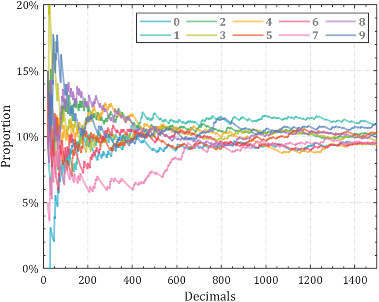
% 获取pi前1500位小数
Pi=getPi(1500);
% 计算比例变化
Ratio=cumsum(Pi==(0:9)',2);
Ratio=Ratio./sum(Ratio);
D=1:length(Ratio);
% 配色列表
CM=[20,164,199;43,187,170;53,165,81;189,190,28;248,167,22;
232,74,27;244,57,99;240,118,177;168,109,195;78,125,187]./255;
hold on
% 循环绘图
for i=1:10
plot(D(20:end),Ratio(i,20:end),'Color',[CM(i,:),.6],'LineWidth',1.8)
end
% 坐标区域修饰
ax=gca;box on;grid on
ax.YLim=[0,.2];
ax.YTick=0:.05:.2;
ax.XTick=0:200:1400;
ax.YTickLabel={'0%','5%','10%','15%','20%'};
ax.XMinorTick='on';
ax.YMinorTick='on';
ax.LineWidth=.8;
ax.GridLineStyle='-.';
ax.FontName='Cambria';
ax.FontSize=11;
ax.XLabel.String='Decimals';
ax.YLabel.String='Proportion';
ax.XLabel.FontSize=13;
ax.YLabel.FontSize=13;
% 绘制图例并修饰
lgdHdl=legend(num2cell('0123456789'));
lgdHdl.NumColumns=5;
lgdHdl.FontWeight='bold';
lgdHdl.FontSize=11;
lgdHdl.TextColor=[.5,.5,.5];
3 stacked area diagram
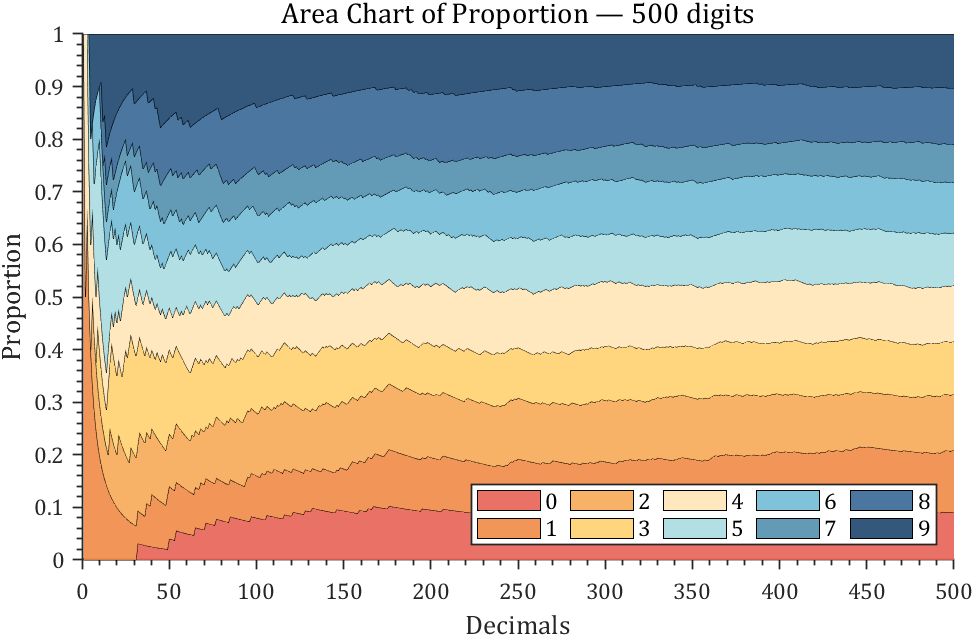
% 获取pi前500位小数
Pi=getPi(500);
% 计算比例变化
Ratio=cumsum(Pi==(0:9)',2);
Ratio=Ratio./sum(Ratio);
% 配色列表
CM=[231,98,84;239,138,71;247,170,88;255,208,111;255,230,183;
170,220,224;114,188,213;82,143,173;55,103,149;30,70,110]./255;
% 绘制堆叠面积图
hold on
areaHdl=area(Ratio');
for i=1:10
areaHdl(i).FaceColor=CM(i,:);
areaHdl(i).FaceAlpha=.9;
end
% 图窗和坐标区域修饰
set(gcf,'Position',[200,100,720,420]);
ax=gca;
ax.YLim=[0,1];
ax.XMinorTick='on';
ax.YMinorTick='on';
ax.LineWidth=.8;
ax.FontName='Cambria';
ax.FontSize=11;
ax.TickDir='out';
ax.XLabel.String='Decimals';
ax.YLabel.String='Proportion';
ax.XLabel.FontSize=13;
ax.YLabel.FontSize=13;
ax.Title.String='Area Chart of Proportion — 500 digits';
ax.Title.FontSize=14;
% 绘制图例并修饰
lgdHdl=legend(num2cell('0123456789'));
lgdHdl.NumColumns=5;
lgdHdl.FontSize=11;
lgdHdl.Location='southeast';
4 connected stacked bar chart
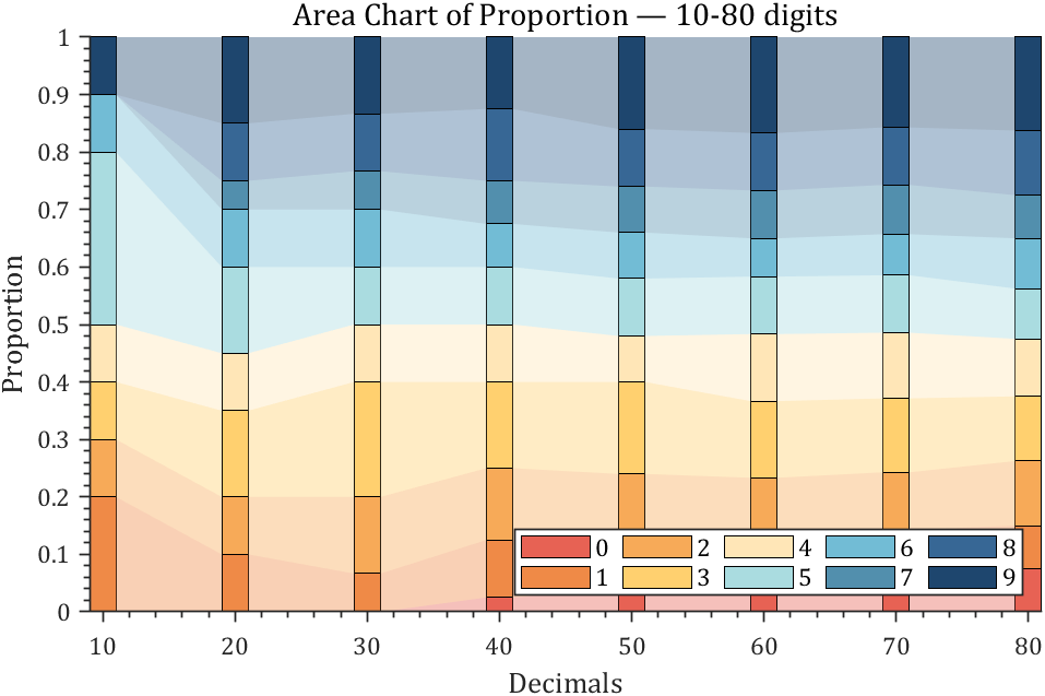
% 获取pi前100位小数
Pi=getPi(100);
% 计算比例变化
Ratio=cumsum(Pi==(0:9)',2);
Ratio=Ratio./sum(Ratio);
X=Ratio(:,10:10:80)';
barHdl=bar(X,'stacked','BarWidth',.2);
CM=[231,98,84;239,138,71;247,170,88;255,208,111;255,230,183;
170,220,224;114,188,213;82,143,173;55,103,149;30,70,110]./255;
for i=1:10
barHdl(i).FaceColor=CM(i,:);
end
% 以下是生成连接的部分
hold on;axis tight
yEndPoints=reshape([barHdl.YEndPoints]',length(barHdl(1).YData),[])';
zeros(1,length(barHdl(1).YData));
yEndPoints=[zeros(1,length(barHdl(1).YData));yEndPoints];
barWidth=barHdl(1).BarWidth;
for i=1:length(barHdl)
for j=1:length(barHdl(1).YData)-1
y1=min(yEndPoints(i,j),yEndPoints(i+1,j));
y2=max(yEndPoints(i,j),yEndPoints(i+1,j));
if y1*y2<0
ty=yEndPoints(find(yEndPoints(i+1,j)*yEndPoints(1:i,j)>=0,1,'last'),j);
y1=min(ty,yEndPoints(i+1,j));
y2=max(ty,yEndPoints(i+1,j));
end
y3=min(yEndPoints(i,j+1),yEndPoints(i+1,j+1));
y4=max(yEndPoints(i,j+1),yEndPoints(i+1,j+1));
if y3*y4<0
ty=yEndPoints(find(yEndPoints(i+1,j+1)*yEndPoints(1:i,j+1)>=0,1,'last'),j+1);
y3=min(ty,yEndPoints(i+1,j+1));
y4=max(ty,yEndPoints(i+1,j+1));
end
fill([j+.5.*barWidth,j+1-.5.*barWidth,j+1-.5.*barWidth,j+.5.*barWidth],...
[y1,y3,y4,y2],barHdl(i).FaceColor,'FaceAlpha',.4,'EdgeColor','none');
end
end
% 图窗和坐标区域修饰
set(gcf,'Position',[200,100,720,420]);
ax=gca;box off
ax.YLim=[0,1];
ax.XMinorTick='on';
ax.YMinorTick='on';
ax.LineWidth=.8;
ax.FontName='Cambria';
ax.FontSize=11;
ax.TickDir='out';
ax.XTickLabel={'10','20','30','40','50','60','70','80'};
ax.XLabel.String='Decimals';
ax.YLabel.String='Proportion';
ax.XLabel.FontSize=13;
ax.YLabel.FontSize=13;
ax.Title.String='Area Chart of Proportion — 10-80 digits';
ax.Title.FontSize=14;
% 绘制图例并修饰
lgdHdl=legend(barHdl,num2cell('0123456789'));
lgdHdl.NumColumns=5;
lgdHdl.FontSize=11;
lgdHdl.Location='southeast';
5 bichord chart
Need to use this tool:

% 构建连接矩阵
dataMat=zeros(10,10);
Pi=getPi(1001);
for i=1:1000
dataMat(Pi(i)+1,Pi(i+1)+1)=dataMat(Pi(i)+1,Pi(i+1)+1)+1;
end
BCC=biChordChart(dataMat,'Arrow','on','Label',num2cell('0123456789'));
BCC=BCC.draw();
% 添加刻度
BCC.tickState('on')
% 修改字体,字号及颜色
BCC.setFont('FontName','Cambria','FontSize',17)
set(gcf,'Position',[200,100,820,820]);
6 Gravity simulation diagram
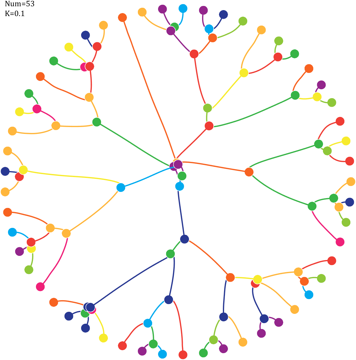
Imagine each decimal as a small ball with a mass of
For example, if , the weight of ball 0 is 1, ball 9 is 1.2589, the initial velocity of the ball is 0, and it is attracted by other balls. Gravity follows the inverse square law, and if the balls are close enough, they will collide and their value will become

After adding, take the mod, add the velocity direction proportionally, and recalculate the weight.
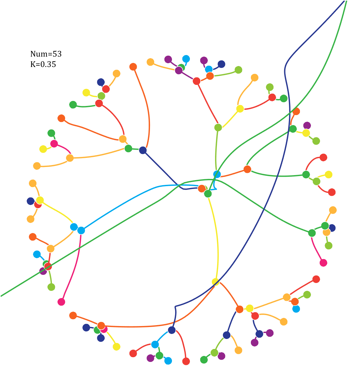
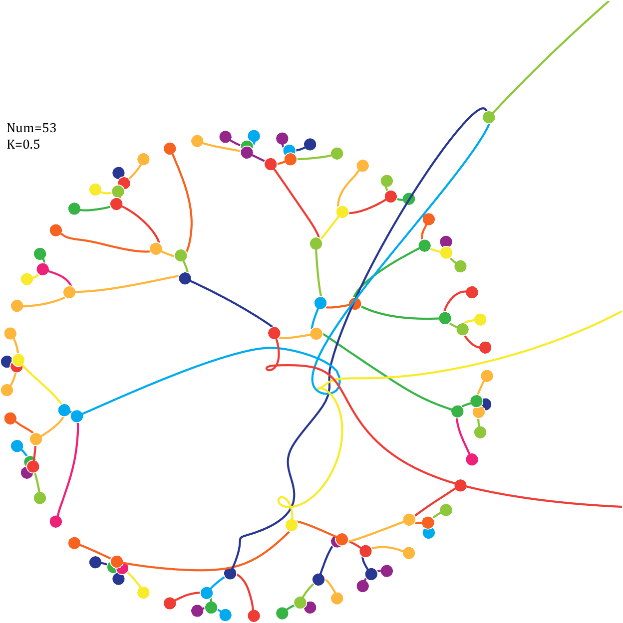
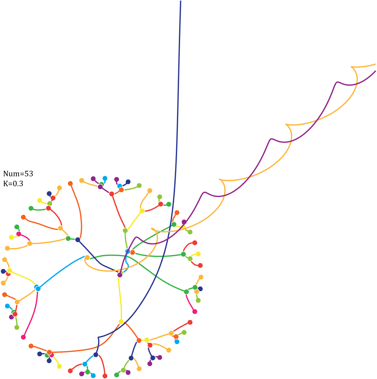
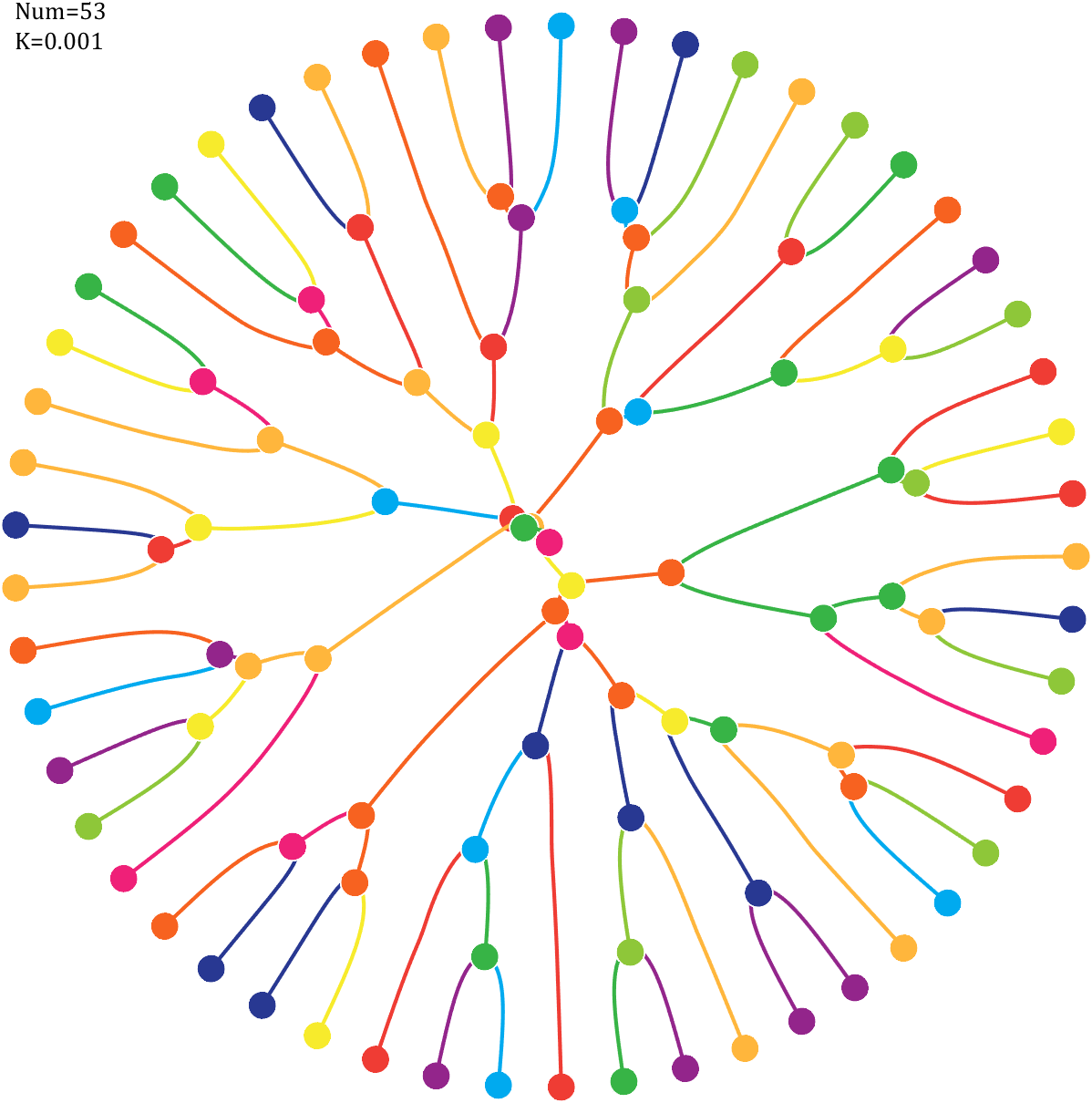
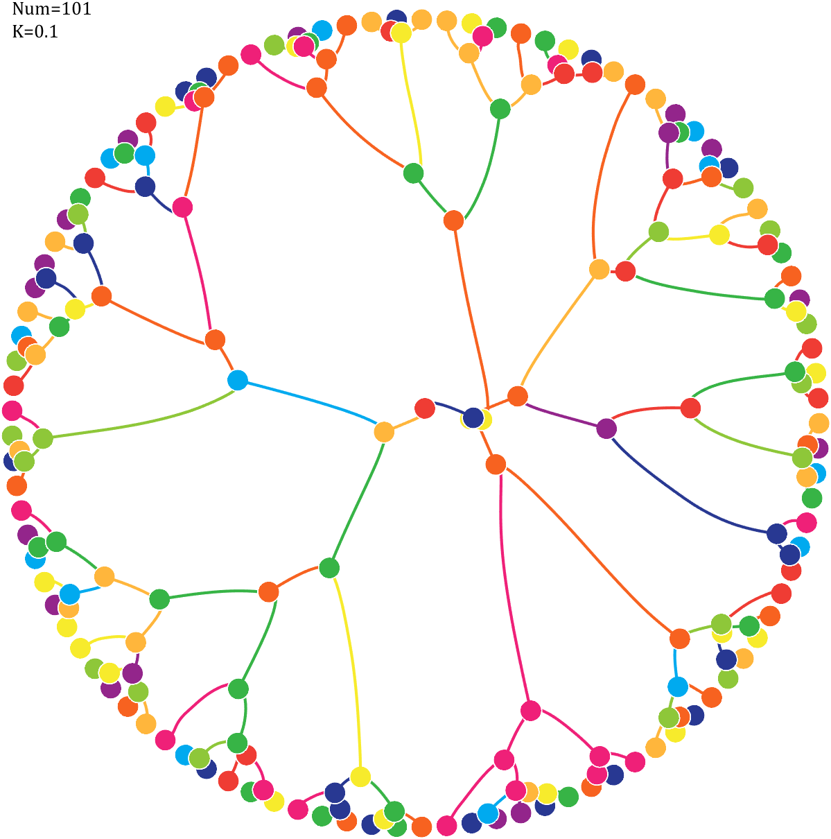
Pi=[3,getPi(71)];K=.18;
% 基础配置
CM=[239,32,120;239,60,52;247,98,32;255,182,60;247,235,44;
142,199,57;55,180,70;0,170,239;40,56,146;147,37,139]./255;
T=linspace(0,2*pi,length(Pi)+1)';
T=T(1:end-1);
ct=linspace(0,2*pi,100);
cx=cos(ct).*.027;
cy=sin(ct).*.027;
% 初始数据
Pi=Pi(:);
N=Pi;
X=cos(T);Y=sin(T);
VX=T.*0;VY=T.*0;
PX=X;PY=Y;
% 未碰撞时初始质量
getM=@(x)(x+1).^K;
M=getM(N);
% 绘制初始圆圈
hold on
for i=1:length(N)
fill(cx+X(i),cy+Y(i),CM(N(i)+1,:),'EdgeColor','w','LineWidth',1)
end
for k=1:800
% 计算加速度
Rn2=1./squareform(pdist([X,Y])).^2;
Rn2(eye(length(X))==1)=0;
MRn2=Rn2.*(M');
AX=X'-X;AY=Y'-Y;
normXY=sqrt(AX.^2+AY.^2);
AX=AX./normXY;AX(eye(length(X))==1)=0;
AY=AY./normXY;AY(eye(length(X))==1)=0;
AX=sum(AX.*MRn2,2)./150000;
AY=sum(AY.*MRn2,2)./150000;
% 计算速度及新位置
VX=VX+AX;X=X+VX;PX=[PX,X];
VY=VY+AY;Y=Y+VY;PY=[PY,Y];
% 检测是否有碰撞
R=squareform(pdist([X,Y]));
R(triu(ones(length(X)))==1)=inf;
[row,col]=find(R<=0.04);
if length(X)==1
break;
end
if ~isempty(row)
% 碰撞的点合为一体
XC=(X(row)+X(col))./2;YC=(Y(row)+Y(col))./2;
VXC=(VX(row).*M(row)+VX(col).*M(col))./(M(row)+M(col));
VYC=(VY(row).*M(row)+VY(col).*M(col))./(M(row)+M(col));
PC=nan(length(row),size(PX,2));
NC=mod(N(row)+N(col),10);
% 删除碰撞点并绘图
uniNum=unique([row;col]);
X(uniNum)=[];VX(uniNum)=[];
Y(uniNum)=[];VY(uniNum)=[];
for i=1:length(uniNum)
plot(PX(uniNum(i),:),PY(uniNum(i),:),'LineWidth',2,'Color',CM(N(uniNum(i))+1,:))
end
PX(uniNum,:)=[];PY(uniNum,:)=[];N(uniNum,:)=[];
% 绘制圆形
for i=1:length(XC)
fill(cx+XC(i),cy+YC(i),CM(NC(i)+1,:),'EdgeColor','w','LineWidth',1)
end
% 补充合体点
X=[X;XC];Y=[Y;YC];VX=[VX;VXC];VY=[VY;VYC];
PX=[PX;PC];PY=[PY;PC];N=[N;NC];M=getM(N);
end
end
for i=1:size(PX,1)
plot(PX(i,:),PY(i,:),'LineWidth',2,'Color',CM(N(i)+1,:))
end
text(-1,1,{['Num=',num2str(length(Pi))];['K=',num2str(K)]},'FontSize',13,'FontName','Cambria')
% 图窗及坐标区域修饰
set(gcf,'Position',[200,100,820,820]);
ax=gca;
ax.Position=[0,0,1,1];
ax.DataAspectRatio=[1,1,1];
ax.XLim=[-1.1,1.1];
ax.YLim=[-1.1,1.1];
ax.XTick=[];
ax.YTick=[];
ax.XColor='none';
ax.YColor='none';
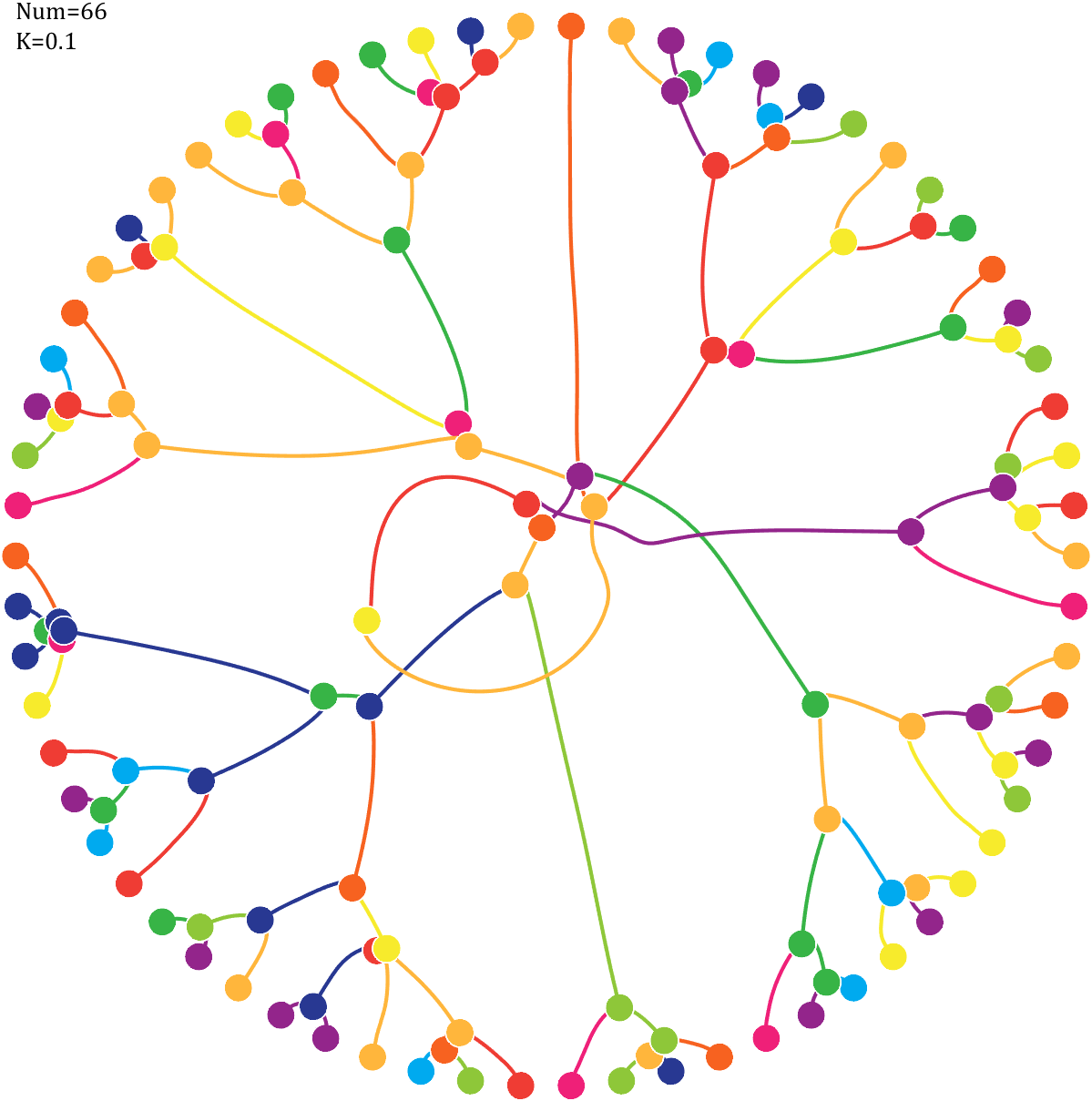
7 forest chart

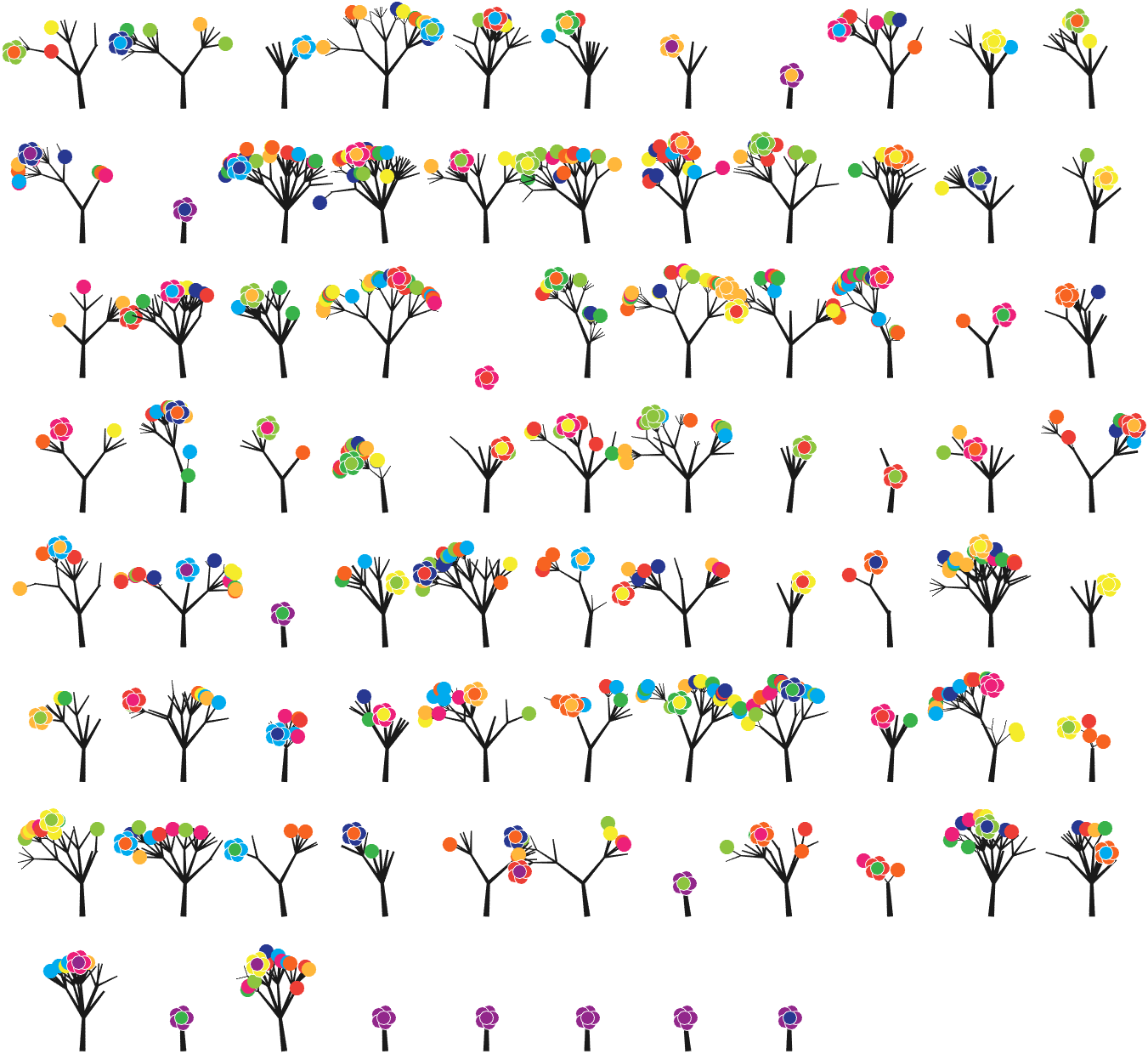
The method comes from
The digits of π are shown as a forest. Each tree in the forest represents the digits of π up to the next 9. The first 10 trees are "grown" from the digit sets 314159, 2653589, 79, 3238462643383279, 50288419, 7169, 39, 9, 3751058209, and 749.
BRANCHES
The first digit of a tree controls how many branches grow from the trunk of the tree. For example, the first tree's first digit is 3, so you see 3 branches growing from the trunk.
The next digit's branches grow from the end of a branch of the previous digit in left-to-right order. This process continues until all the tree's digits have been used up.
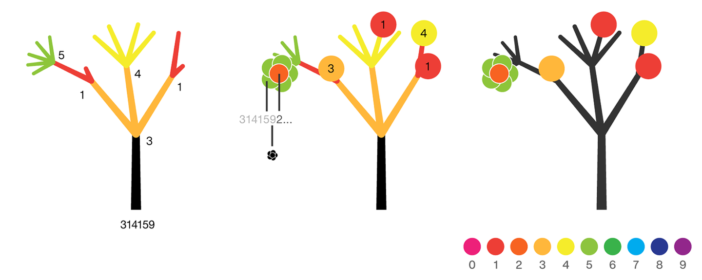
Each tree grows from a set of consecutive digits sampled from the digits of π up to the next 9. The first tree, shown here, grows from 314159. Each of the digits determine how many branches grow at each fork in the tree — the branches here are colored by their corresponding digit to illustrate this. Leaves encode the digits in a left-to-right order. The digit 9 spawns a flower on one of the branches of the previous digit. The branching exception is 0, which terminates the current branch — 0 branches grow!
LEAVES AND FLOWERS
The tree's digits themselves are drawn as circular leaves, color-coded by the digit.
The leaf exception is 9, which causes one of the branches of the previous digit to sprout a flower! The petals of the flower are colored by the digit before the 9 and the center is colored by the digit after the 9, which is on the next tree. This is how the forest propagates.
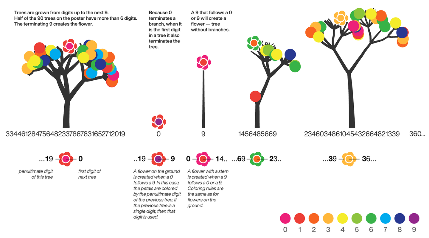
The colors of a flower are determined by the first digit of the next tree and the penultimate digit of the current tree. If the current tree only has one digit, then that digit is used. Leaves are placed at the tips of branches in a left-to-right order — you can "easily" read them off. Additionally, the leaves are distributed within the tree (without disturbing their left-to-right order) to spread them out as much as possible and avoid overlap. This order is deterministic.
The leaf placement exception are the branch set that sprouted the flower. These are not used to grow leaves — the flower needs space!
function PiTree(X,pos,D)
lw=2;
theta=pi/2+(rand(1)-.5).*pi./12;
% 树叶及花朵颜色
CM=[237,32,121;237,62,54;247,99,33;255,183,59;245,236,43;
141,196,63;57,178,74;0,171,238;40,56,145;146,39,139]./255;
hold on
if all(X(1:end-2)==0)
endSet=[pos,pos,theta];
else
kplot(pos(1)+[0,cos(theta)],pos(2)+[0,sin(theta)],lw./.6)
endSet=[pos,pos+[cos(theta),sin(theta)],theta];
% 计算层级
Layer=0;
for i=1:length(X)
Layer=[Layer,ones(1,X(i)).*i];
end
% 计算树枝
if D
for i=1:length(X)-2
if X(i)==0 % 若数值为0则不长树枝
newSet=endSet(1,:);
elseif X(i)==1 % 若数值为1则一长一短两个树枝
tTheta=endSet(1,5);
tTheta=linspace(tTheta+pi/8,tTheta-pi/8,2)'+(rand([2,1])-.5).*pi./8;
newSet=repmat(endSet(1,3:4),[X(i),1]);
newSet=[newSet.*[1;1],newSet+[cos(tTheta),sin(tTheta)].*.7^Layer(i).*[1;.1],tTheta];
else % 其他情况数值为几长几个树枝
tTheta=endSet(1,5);
tTheta=linspace(tTheta+pi/5,tTheta-pi/5,X(i))'+(rand([X(i),1])-.5).*pi./8;
newSet=repmat(endSet(1,3:4),[X(i),1]);
newSet=[newSet,newSet+[cos(tTheta),sin(tTheta)].*.7^Layer(i),tTheta];
end
% 绘制树枝
for j=1:size(newSet,1)
kplot(newSet(j,[1,3]),newSet(j,[2,4]),lw.*.6^Layer(i))
end
endSet=[endSet;newSet];
endSet(1,:)=[];
end
end
end
% 计算叶子和花朵位置
FLSet=endSet(:,3:4);
[~,FLInd]=sort(FLSet(:,1));
FLSet=FLSet(FLInd,:);
[~,tempInd]=sort(rand([1,size(FLSet,1)]));
tempInd=sort(tempInd(1:length(X)-2));
flowerInd=tempInd(randi([1,length(X)-2],[1,1]));
leafInd=tempInd(tempInd~=flowerInd);
% 绘制树叶
for i=1:length(leafInd)
scatter(FLSet(leafInd(i),1),FLSet(leafInd(i),2),70,'filled','CData',CM(X(i)+1,:))
end
% 绘制花朵
for i=1:5
% if ~D
% tC=CM(X(end)+1,:);
% else
% tC=CM(X(end-2)+1,:);
% end
scatter(FLSet(flowerInd,1)+cos(pi*2*i/5).*.18,FLSet(flowerInd,2)+sin(pi*2*i/5).*.18,60,...
'filled','CData',CM(X(end-2)+1,:),'MarkerEdgeColor',[1,1,1])
end
scatter(FLSet(flowerInd,1),FLSet(flowerInd,2),60,'filled','CData',CM(X(end)+1,:),'MarkerEdgeColor',[1,1,1])
drawnow;%axis tight
% =========================================================================
function kplot(XX,YY,LW,varargin)
LW=linspace(LW,LW*.6,10);%+rand(1,20).*LW./10;
XX=linspace(XX(1),XX(2),11)';
XX=[XX(1:end-1),XX(2:end)];
YY=linspace(YY(1),YY(2),11)';
YY=[YY(1:end-1),YY(2:end)];
for ii=1:10
plot(XX(ii,:),YY(ii,:),'LineWidth',LW(ii),'Color',[.1,.1,.1])
end
end
end
main part:
Pi=[3,getPi(800)];
pos9=[0,find(Pi==9)];
set(gcf,'Position',[200,50,900,900],'Color',[1,1,1]);
ax=gca;hold on
ax.Position=[0,0,1,1];
ax.DataAspectRatio=[1,1,1];
ax.XLim=[.5,36];
ax.XTick=[];
ax.YTick=[];
ax.XColor='none';
ax.YColor='none';
for j=1:8
for i=1:11
n=i+(j-1)*11;
if n<=85
tPi=Pi((pos9(n)+1):pos9(n+1)+1);
if length(tPi)>2
PiTree(tPi,[0+i*3,0-j*4],true);
else
PiTree([Pi(pos9(n)),tPi],[0+i*3,0-j*4],false);
end
end
end
end
8 random walk
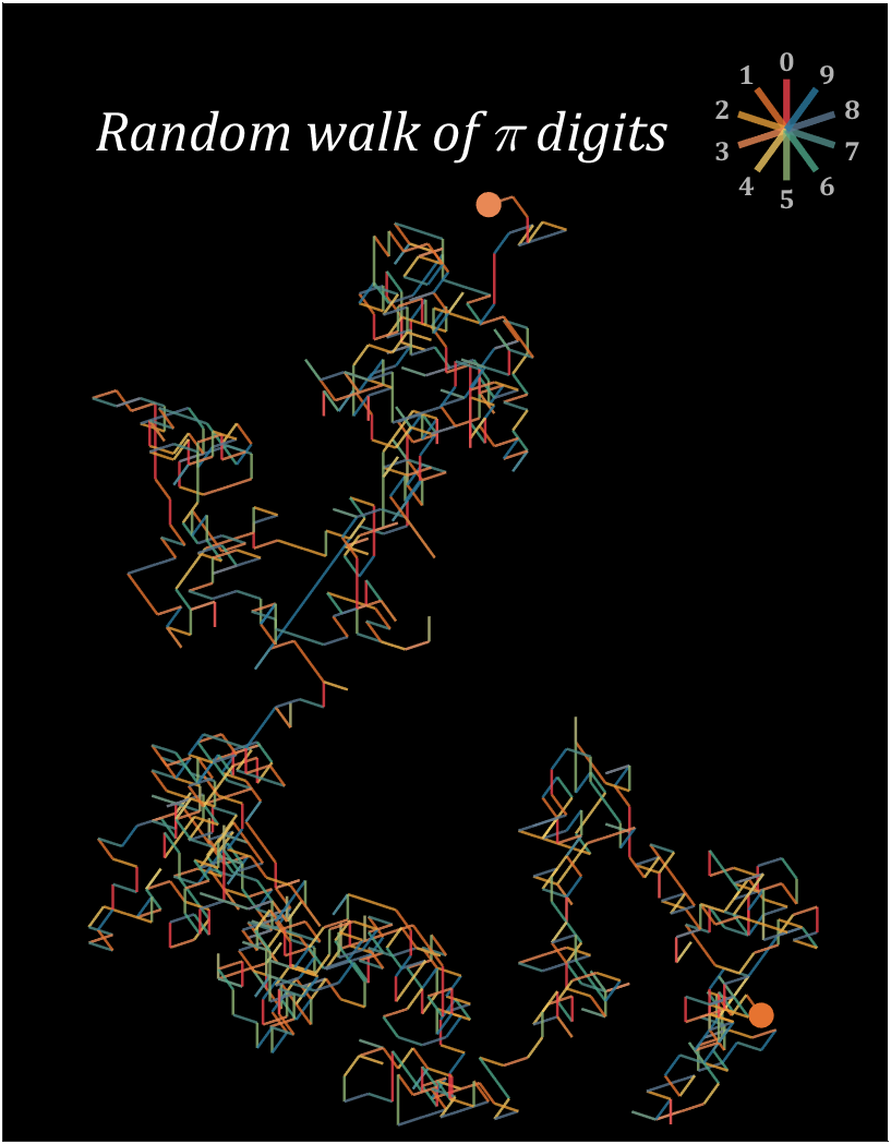
n=1200;
% 获取pi前n位小数
Pi=getPi(n);
CM=[239,65,75;230,115,48;229,158,57;232,136,85;239,199,97;
144,180,116;78,166,136;81,140,136;90,118,142;43,121,159]./255;
hold on
endPoint=[0,0];
t=linspace(0,2*pi,100);
T=linspace(0,2*pi,11)+pi/2;
fill(endPoint(1)+cos(t).*.5,endPoint(2)+sin(t).*.5,CM(Pi(1)+1,:),'EdgeColor','none')
for i=1:n
theta=T(Pi(i)+1);
plot(endPoint(1)+[0,cos(theta)],endPoint(2)+[0,sin(theta)],'Color',[CM(Pi(i)+1,:),.8],'LineWidth',1.2);
endPoint=endPoint+[cos(theta),sin(theta)];
end
fill(endPoint(1)+cos(t).*.5,endPoint(2)+sin(t).*.5,CM(Pi(n)+1,:),'EdgeColor','none')
% 图窗和坐标区域修饰
set(gcf,'Position',[200,100,820,820]);
ax=gca;
ax.XTick=[];
ax.YTick=[];
ax.Color=[0,0,0];
ax.DataAspectRatio=[1,1,1];
ax.XLim=[-30,5];
ax.YLim=[-5,40];
% 绘制图例
endPoint=[1,35];
for i=1:10
theta=T(i);
plot(endPoint(1)+[0,cos(theta).*2],endPoint(2)+[0,sin(theta).*2],'Color',[CM(i,:),.8],'LineWidth',3);
text(endPoint(1)+cos(theta).*2.7,endPoint(2)+sin(theta).*2.7,num2str(i-1),'Color',[1,1,1].*.7,...
'FontSize',12,'FontWeight','bold','FontName','Cambria','HorizontalAlignment','center')
end
text(-15,35,'Random walk of \pi digits','Color',[1,1,1],'FontName','Cambria',...
'HorizontalAlignment','center','FontSize',25,'FontAngle','italic')
9 grid chart
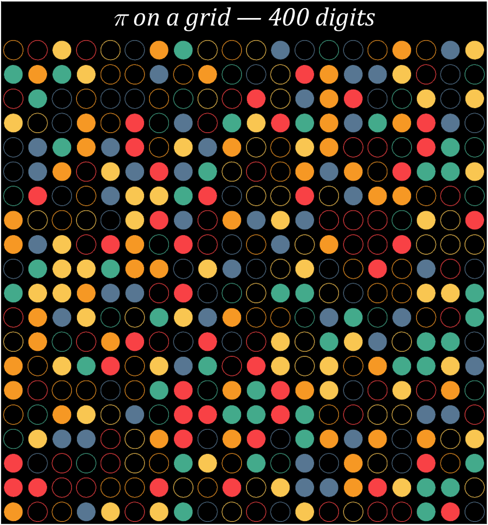
Pi=[3,getPi(399)];
% 配色数据
CM=[248,65,69;246,152,36;249,198,81;67,170,139;87,118,146]./255;
% 绘制圆圈
hold on
t=linspace(0,2*pi,100);
x=cos(t).*.8.*.5;
y=sin(t).*.8.*.5;
for i=1:400
[col,row]=ind2sub([20,20],i);
if mod(Pi(i),2)==0
fill(x+col,y+row,CM(round((Pi(i)+1)/2),:),'LineWidth',1,'EdgeAlpha',.8)
else
fill(x+col,y+row,[0,0,0],'EdgeColor',CM(round((Pi(i)+1)/2),:),'LineWidth',1,'EdgeAlpha',.7)
end
end
text(10.5,-.4,'\pi on a grid — 400 digits','Color',[1,1,1],'FontName','Cambria',...
'HorizontalAlignment','center','FontSize',25,'FontAngle','italic')
% 图窗和坐标区域修饰
set(gcf,'Position',[200,100,820,820]);
ax=gca;
ax.YDir='reverse';
ax.XLim=[.5,20.5];
ax.YLim=[-1,20.5];
ax.XTick=[];
ax.YTick=[];
ax.Color=[0,0,0];
ax.DataAspectRatio=[1,1,1];
10 scale grid diagram
Let's still put the numbers in the form of circles, but the difference is that six numbers are grouped together, and the pure purple circle at the end is the six 9s that we are familiar with decimal places 762-767
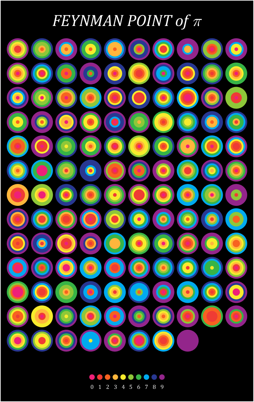
Pi=[3,getPi(767)];
% 762-767
% 配色数据
CM=[239,32,120;239,60,52;247,98,32;255,182,60;247,235,44;
142,199,57;55,180,70;0,170,239;40,56,146;147,37,139]./255;
% 绘制圆圈
hold on
t=linspace(0,2*pi,100);
x=cos(t).*.9.*.5;
y=sin(t).*.9.*.5;
for i=1:6:length(Pi)
n=round((i-1)/6+1);
[col,row]=ind2sub([10,13],n);
tNum=Pi(i:i+5);
numNum=find([diff(sort(tNum)),1]);
numNum=[numNum(1),diff(numNum)];
cumNum=cumsum(numNum);
uniNum=unique(tNum);
for j=length(cumNum):-1:1
fill(x./6.*cumNum(j)+col,y./6.*cumNum(j)+row,CM(uniNum(j)+1,:),'EdgeColor','none')
end
end
% 绘制图例
for i=1:10
fill(x./4+5.5+(i-5.5)*.32,y./4+14.5,CM(i,:),'EdgeColor','none')
text(5.5+(i-5.5)*.32,14.9,num2str(i-1),'Color',[1,1,1],'FontSize',...
9,'FontName','Cambria','HorizontalAlignment','center')
end
text(5.5,-.2,'FEYNMAN POINT of \pi','Color',[1,1,1],'FontName','Cambria',...
'HorizontalAlignment','center','FontSize',25,'FontAngle','italic')
% 图窗和坐标区域修饰
set(gcf,'Position',[200,100,600,820]);
ax=gca;
ax.YDir='reverse';
ax.Position=[0,0,1,1];
ax.XLim=[.3,10.7];
ax.YLim=[-1,15.5];
ax.XTick=[];
ax.YTick=[];
ax.Color=[0,0,0];
ax.DataAspectRatio=[1,1,1];
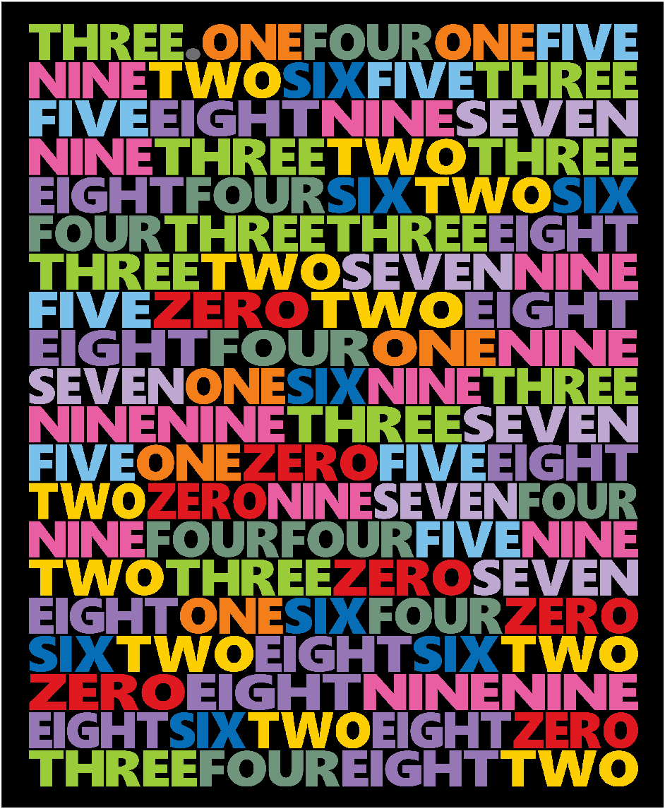
11 text chart

First, write a code to generate an image of each letter:
function getLogo
if ~exist('image','dir')
mkdir('image\')
end
logoSet=['.',char(65:90)];
for i=1:27
figure();
ax=gca;
ax.XLim=[-1,1];
ax.YLim=[-1,1];
ax.XColor='none';
ax.YColor='none';
ax.DataAspectRatio=[1,1,1];
logo=logoSet(i);
hold on
text(0,0,logo,'HorizontalAlignment','center','FontSize',320,'FontName','Segoe UI Black')
exportgraphics(ax,['image\',logo,'.png'])
close
end
dotPic=imread('image\..png');
newDotPic=uint8(ones([400,size(dotPic,2),3]).*255);
newDotPic(end-size(dotPic,1)+1:end,:,1)=dotPic(:,:,1);
newDotPic(end-size(dotPic,1)+1:end,:,2)=dotPic(:,:,2);
newDotPic(end-size(dotPic,1)+1:end,:,3)=dotPic(:,:,3);
imwrite(newDotPic,'image\..png')
S=20;
for i=1:27
logo=logoSet(i);
tPic=imread(['image\',logo,'.png']);
sz=size(tPic,[1,2]);
sz=round(sz./sz(1).*400);
tPic=imresize(tPic,sz);
tBox=uint8(255.*ones(size(tPic,[1,2])+S));
tBox(S+1:S+size(tPic,1),S+1:S+size(tPic,2))=tPic(:,:,1);
imwrite(cat(3,tBox,tBox,tBox),['image\',logo,'.png'])
end
end
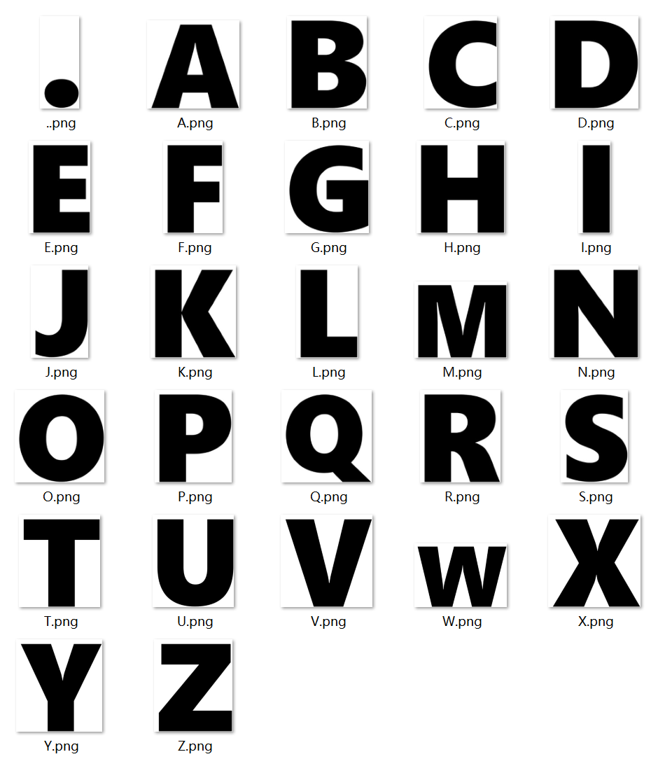
Pi=[3,-1,getPi(150)];
CM=[109,110,113;224,25,33;244,126,26;253,207,2;154,203,57;111,150,124;
121,192,235;6,109,183;190,168,209;151,118,181;233,93,163]./255;
ST={'.','ZERO','ONE','TWO','THREE','FOUR','FIVE','SIX','SEVEN','EIGHT','NINE'};
n=1;
hold on
% 循环绘制字母
for i=1:20%:10
STList='';
NMList=[];
PicListR=uint8(zeros(400,0));
PicListG=uint8(zeros(400,0));
PicListB=uint8(zeros(400,0));
% PicListA=uint8(zeros(400,0));
for j=1:6
STList=[STList,ST{Pi(n)+2}];
NMList=[NMList,ones(size(ST{Pi(n)+2})).*(Pi(n)+2)];
n=n+1;
if length(STList)>15&&length(STList)+length(ST{Pi(n)+2})>20
break;
end
end
for k=1:length(STList)
tPic=imread(['image\',STList(k),'.png']);
% PicListA=[PicListA,tPic(:,:,1)];
PicListR=[PicListR,(255-tPic(:,:,1)).*CM(NMList(k),1)];
PicListG=[PicListG,(255-tPic(:,:,2)).*CM(NMList(k),2)];
PicListB=[PicListB,(255-tPic(:,:,3)).*CM(NMList(k),3)];
end
PicList=cat(3,PicListR,PicListG,PicListB);
image([-1200,1200],[0,150]-(i-1)*150,flipud(PicList))
end
% 图窗及坐标区域修饰
set(gcf,'Position',[200,100,600,820]);
ax=gca;
ax.DataAspectRatio=[1,1,1];
ax.XLim=[-1300,1300];
ax.Position=[0,0,1,1];
ax.XTick=[];
ax.YTick=[];
ax.Color=[0,0,0];
ax.YLim=[-19*150-80,230];
12 spiral chart
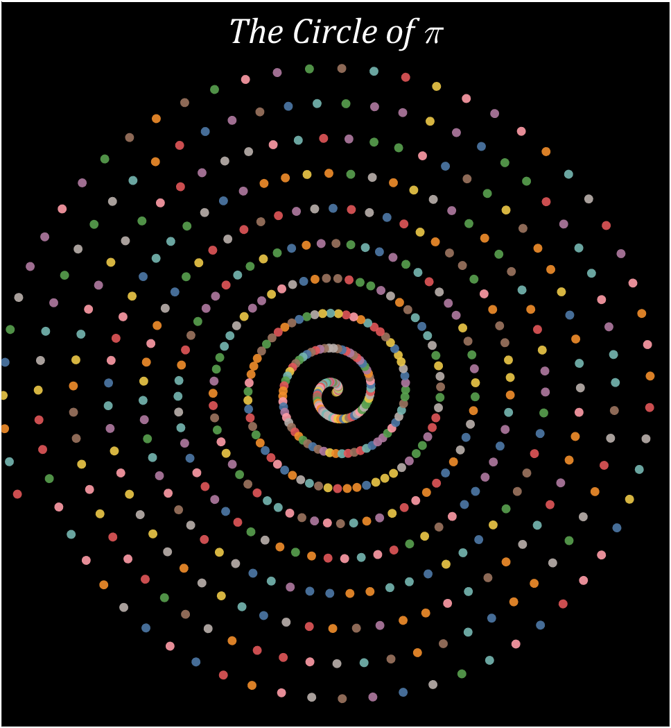
Pi=getPi(600);
% 配色列表
CM=[78,121,167;242,142,43;225,87,89;118,183,178;89,161,79;
237,201,72;176,122,161;255,157,167;156,117,95;186,176,172]./255;
% 绘制圆圈
hold on
t=linspace(0,2*pi,100);
x=cos(t).*.8;
y=sin(t).*.8;
for i=1:600
X=i.*cos(i./10)./10;
Y=i.*sin(i./10)./10;
fill(X+x,Y+y,CM(Pi(i)+1,:),'EdgeColor','none','FaceAlpha',.9)
end
text(0,65,'The Circle of \pi','Color',[1,1,1],'FontName','Cambria',...
'HorizontalAlignment','center','FontSize',25,'FontAngle','italic')
% 图窗和坐标区域修饰
set(gcf,'Position',[200,100,820,820]);
ax=gca;
ax.XLim=[-60,60];
ax.YLim=[-60,70];
ax.XTick=[];
ax.YTick=[];
ax.Color=[0,0,0];
ax.DataAspectRatio=[1,1,1];
13 Archimedean spiral diagram
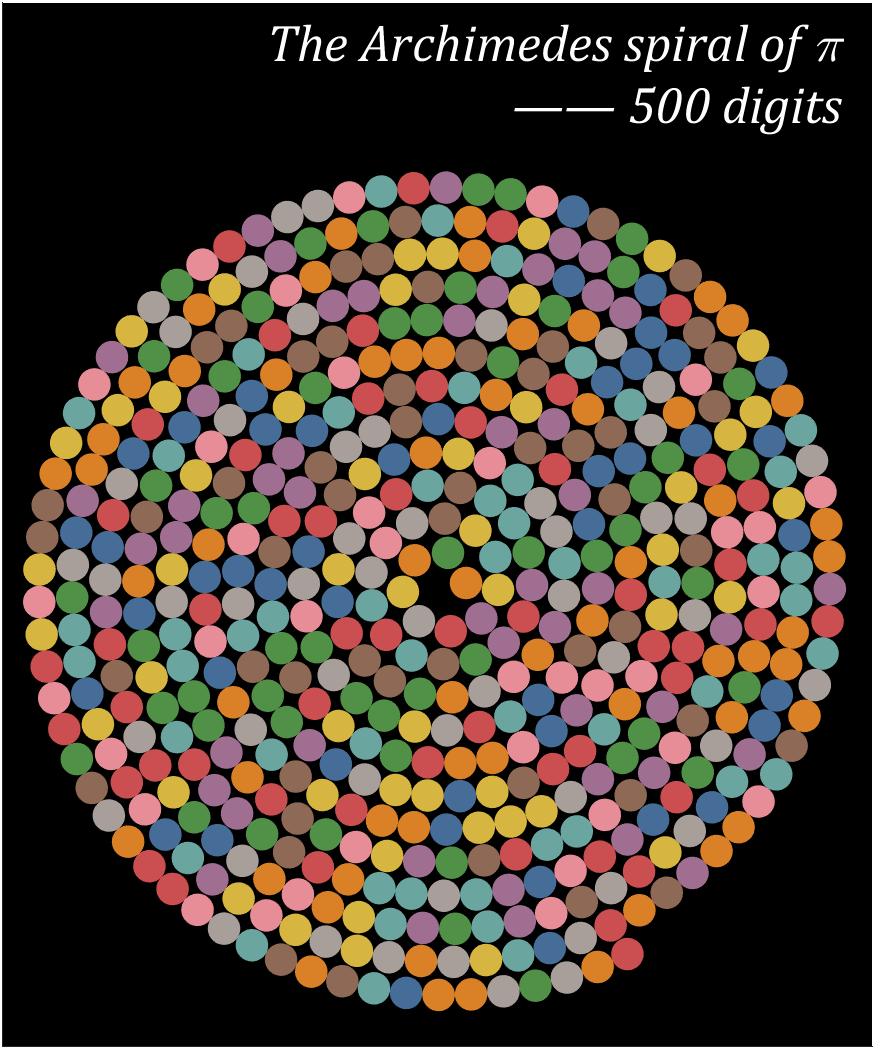
a=1;b=.227;
Pi=getPi(500);
% 配色列表
CM=[78,121,167;242,142,43;225,87,89;118,183,178;89,161,79;
237,201,72;176,122,161;255,157,167;156,117,95;186,176,172]./255;
% 绘制圆圈
hold on
T=0;R=1;
t=linspace(0,2*pi,100);
x=cos(t).*.7;
y=sin(t).*.7;
for i=1:500
X=R.*cos(T);Y=R.*sin(T);
fill(X+x,Y+y,CM(Pi(i)+1,:),'EdgeColor','none','FaceAlpha',.9)
T=T+1./R.*1.4;
R=a+b*T;
end
text(17.25,22,{'The Archimedes spiral of \pi';'—— 500 digits'},...
'Color',[1,1,1],'FontName','Cambria',...
'HorizontalAlignment','right','FontSize',25,'FontAngle','italic')
% 图窗和坐标区域修饰
set(gcf,'Position',[200,100,820,820]);
ax=gca;
ax.XLim=[-19,18.5];
ax.YLim=[-20,25];
ax.XTick=[];
ax.YTick=[];
ax.Color=[0,0,0];
ax.DataAspectRatio=[1,1,1];
14 proportional Archimedean spiral diagram
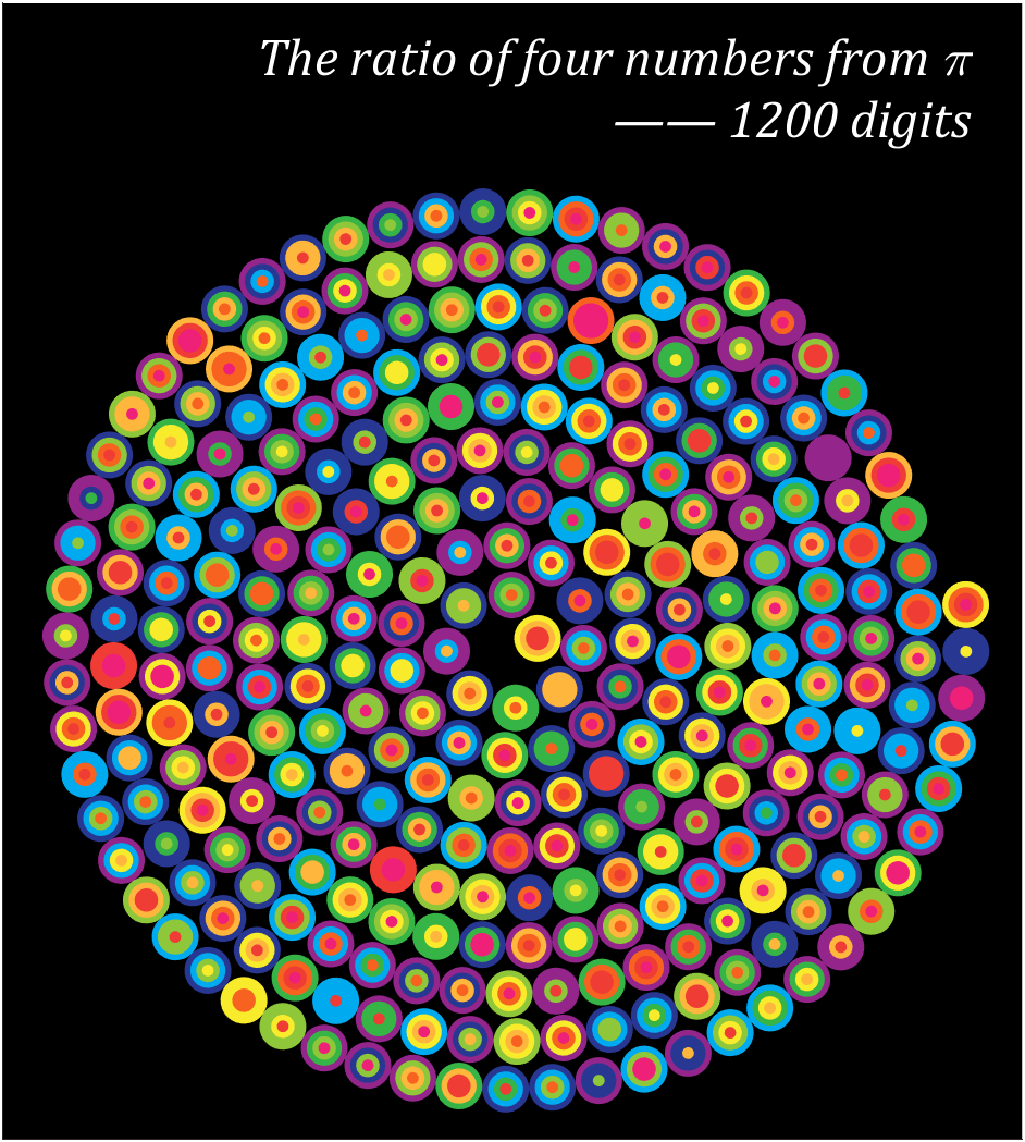
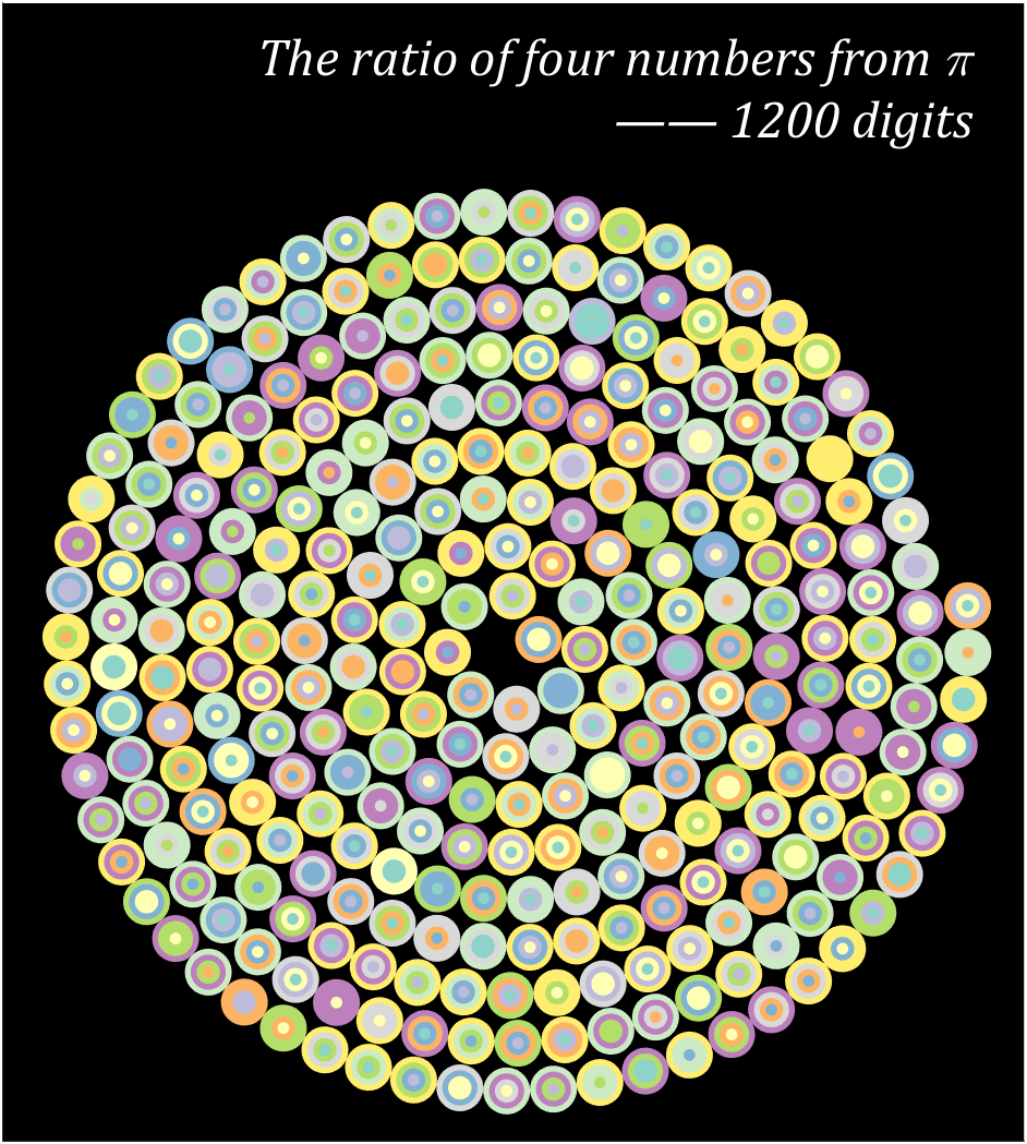
Pi=[3,getPi(1199)];
% 配色数据
CM=[239,32,120;239,60,52;247,98,32;255,182,60;247,235,44;
142,199,57;55,180,70;0,170,239;40,56,146;147,37,139]./255;
% CM=slanCM(184,10);
% 绘制圆圈
hold on
T=0;R=1;
t=linspace(0,2*pi,100);
x=cos(t).*.7;
y=sin(t).*.7;
for i=1:4:length(Pi)
X=R.*cos(T);Y=R.*sin(T);
tNum=Pi(i:i+3);
numNum=find([diff(sort(tNum)),1]);
numNum=[numNum(1),diff(numNum)];
cumNum=cumsum(numNum);
uniNum=unique(tNum);
for j=length(cumNum):-1:1
fill(x./4.*cumNum(j)+X,y./4.*cumNum(j)+Y,CM(uniNum(j)+1,:),'EdgeColor','none')
end
T=T+1./R.*1.4;
R=a+b*T;
end
text(14,16.5,{'The ratio of four numbers from \pi';'—— 1200 digits'},...
'Color',[1,1,1],'FontName','Cambria',...
'HorizontalAlignment','right','FontSize',23,'FontAngle','italic')
% 图窗和坐标区域修饰
set(gcf,'Position',[200,100,820,820]);
ax=gca;
ax.XLim=[-15,15.5];
ax.YLim=[-15,19];
ax.XTick=[];
ax.YTick=[];
ax.Color=[0,0,0];
ax.DataAspectRatio=[1,1,1];
15 graph
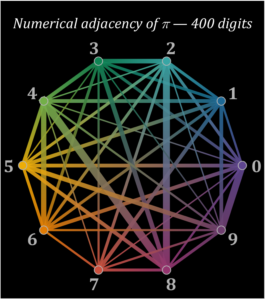
% 构建连接矩阵
corrMat=zeros(10,10);
Pi=getPi(401);
for i=1:400
corrMat(Pi(i)+1,Pi(i+1)+1)=corrMat(Pi(i)+1,Pi(i+1)+1)+1;
end
% 配色列表
colorList=[0.3725 0.2745 0.5647
0.1137 0.4118 0.5882
0.2196 0.6510 0.6471
0.0588 0.5216 0.3294
0.4510 0.6863 0.2824
0.9294 0.6784 0.0314
0.8824 0.4863 0.0196
0.8000 0.3137 0.2431
0.5804 0.2039 0.4314
0.4353 0.2510 0.4392];
t=linspace(0,2*pi,11);t=t(1:10)';
posXY=[cos(t),sin(t)];
maxWidth=max(corrMat(corrMat>0));
minWidth=min(corrMat(corrMat>0));
ttList=linspace(0,1,3)';
% 循环绘图
hold on
for i=1:size(corrMat,1)
for j=i+1:size(corrMat,2)
if corrMat(i,j)>0
tW=(corrMat(i,j)-minWidth)./(maxWidth-minWidth);
colorData=(1-ttList).*colorList(i,:)+ttList.*colorList(j,:);
CData(:,:,1)=colorData(:,1);
CData(:,:,2)=colorData(:,2);
CData(:,:,3)=colorData(:,3);
% 绘制连线
fill(linspace(posXY(i,1),posXY(j,1),3),...
linspace(posXY(i,2),posXY(j,2),3),[0,0,0],'LineWidth',tW.*12+1,...
'CData',CData,'EdgeColor','interp','EdgeAlpha',.7,'FaceAlpha',.7)
end
end
% 绘制圆点
scatter(posXY(i,1),posXY(i,2),200,'filled','LineWidth',1.2,...
'MarkerFaceColor',colorList(i,:),'MarkerEdgeColor',[.7,.7,.7]);
text(posXY(i,1).*1.13,posXY(i,2).*1.13,num2str(i-1),'Color',[1,1,1].*.7,...
'FontSize',30,'FontWeight','bold','FontName','Cambria','HorizontalAlignment','center')
end
text(0,1.3,'Numerical adjacency of \pi — 400 digits','Color',[1,1,1],'FontName','Cambria',...
'HorizontalAlignment','center','FontSize',25,'FontAngle','italic')
% 图窗和坐标区域修饰
set(gcf,'Position',[200,100,820,820]);
ax=gca;
ax.XLim=[-1.2,1.2];
ax.YLim=[-1.21,1.5];
ax.XTick=[];
ax.YTick=[];
ax.Color=[0,0,0];
ax.DataAspectRatio=[1,1,1];
16 circos chart
Need to use this tool:
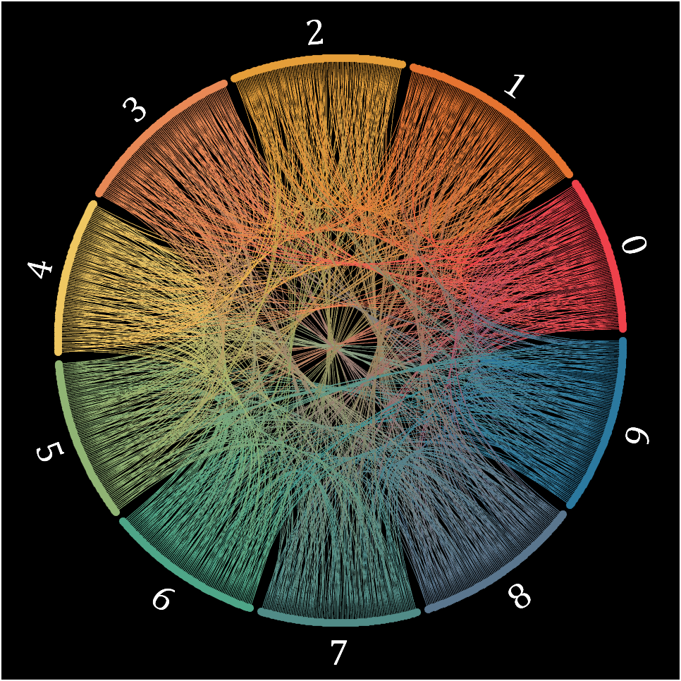
Class=getPi(1001)+1;
Data=diag(ones(1,1000),-1);
className={'0','1','2','3','4','5','6','7','8','9'};
colorOrder=[239,65,75;230,115,48;229,158,57;232,136,85;239,199,97;
144,180,116;78,166,136;81,140,136;90,118,142;43,121,159]./255;
CC=circosChart(Data,Class,'ClassName',className,'ColorOrder',colorOrder);
CC=CC.draw();
ax=gca;
ax.Color=[0,0,0];
CC.setClassLabel('Color',[1,1,1],'FontSize',25,'FontName','Cambria')
CC.setLine('LineWidth',.7)
YOU CAN GET ALL CODE HERE:
Mathworks has always had quality documentation but in 2023, the documentation quality fell. Will this improve in 2024?
Hi
I have Matlab 2015b installed and if I try:
ones(2,3,4)+ones(2,3)
of course I get an error. But my student has R2023b installed and she gets a 2x3x4 matrix as a result, with all elements = 2.
How is it possible?
Thanks
A
