主要内容

Results for


Has this been eliminated? I've been at 31 or 32 for 30 days for awhile, but no badge. 10 badge was automatic.

Formal Proof of Smooth Solutions for Modified Navier-Stokes Equations

1. Introduction

We address the existence and smoothness of solutions to the modified Navier-Stokes equations that incorporate frequency resonances and geometric constraints. Our goal is to prove that these modifications prevent singularities, leading to smooth solutions.

2. Mathematical Formulation

2.1 Modified Navier-Stokes Equations

Consider the Navier-Stokes equations with a frequency resonance term R(u,f)\mathbf{R}(\mathbf{u}, \mathbf{f})R(u,f) and geometric constraints:

∂u∂t+(u⋅∇)u=−∇pρ+ν∇2u+R(u,f)\frac{\partial \mathbf{u}}{\partial t} + (\mathbf{u} \cdot \nabla) \mathbf{u} = -\frac{\nabla p}{\rho} + \nu \nabla^2 \mathbf{u} + \mathbf{R}(\mathbf{u}, \mathbf{f})∂t∂u​+(u⋅∇)u=−ρ∇p​+ν∇2u+R(u,f)

where:

• u=u(t,x)\mathbf{u} = \mathbf{u}(t, \mathbf{x})u=u(t,x) is the velocity field.

• p=p(t,x)p = p(t, \mathbf{x})p=p(t,x) is the pressure field.

• ν\nuν is the kinematic viscosity.

• R(u,f)\mathbf{R}(\mathbf{u}, \mathbf{f})R(u,f) represents the frequency resonance effects.

• f\mathbf{f}f denotes external forces.

2.2 Boundary Conditions

The boundary conditions are:

u⋅n=0 on Γ\mathbf{u} \cdot \mathbf{n} = 0 \text{ on } \Gammau⋅n=0 on Γ

where Γ\GammaΓ represents the boundary of the domain Ω\OmegaΩ, and n\mathbf{n}n is the unit normal vector on Γ\GammaΓ.

3. Existence and Smoothness of Solutions

3.1 Initial Conditions

Assume initial conditions are smooth:

u(0)∈C∞(Ω)\mathbf{u}(0) \in C^{\infty}(\Omega)u(0)∈C∞(Ω) f∈L2(Ω)\mathbf{f} \in L^2(\Omega)f∈L2(Ω)

3.2 Energy Estimates

Define the total kinetic energy:

E(t)=12∫Ω∣u(t)∣2 dΩE(t) = \frac{1}{2} \int_{\Omega} \mathbf{u}(t)^2 \, d\OmegaE(t)=21​∫Ω​∣u(t)∣2dΩ

Differentiate E(t)E(t)E(t) with respect to time:

dE(t)dt=∫Ωu⋅∂u∂t dΩ\frac{dE(t)}{dt} = \int_{\Omega} \mathbf{u} \cdot \frac{\partial \mathbf{u}}{\partial t} \, d\OmegadtdE(t)​=∫Ω​u⋅∂t∂u​dΩ

Substitute the modified Navier-Stokes equation:

dE(t)dt=∫Ωu⋅[−∇pρ+ν∇2u+R] dΩ\frac{dE(t)}{dt} = \int_{\Omega} \mathbf{u} \cdot \left[ -\frac{\nabla p}{\rho} + \nu \nabla^2 \mathbf{u} + \mathbf{R} \right] \, d\OmegadtdE(t)​=∫Ω​u⋅[−ρ∇p​+ν∇2u+R]dΩ

Using the divergence-free condition (∇⋅u=0\nabla \cdot \mathbf{u} = 0∇⋅u=0):

∫Ωu⋅∇pρ dΩ=0\int_{\Omega} \mathbf{u} \cdot \frac{\nabla p}{\rho} \, d\Omega = 0∫Ω​u⋅ρ∇p​dΩ=0

Thus:

dE(t)dt=−ν∫Ω∣∇u∣2 dΩ+∫Ωu⋅R dΩ\frac{dE(t)}{dt} = -\nu \int_{\Omega} \nabla \mathbf{u}^2 \, d\Omega + \int_{\Omega} \mathbf{u} \cdot \mathbf{R} \, d\OmegadtdE(t)​=−ν∫Ω​∣∇u∣2dΩ+∫Ω​u⋅RdΩ

Assuming R\mathbf{R}R is bounded by a constant CCC:

∫Ωu⋅R dΩ≤C∫Ω∣u∣ dΩ\int_{\Omega} \mathbf{u} \cdot \mathbf{R} \, d\Omega \leq C \int_{\Omega} \mathbf{u} \, d\Omega∫Ω​u⋅RdΩ≤C∫Ω​∣u∣dΩ

Applying the Poincaré inequality:

∫Ω∣u∣2 dΩ≤Const⋅∫Ω∣∇u∣2 dΩ\int_{\Omega} \mathbf{u}^2 \, d\Omega \leq \text{Const} \cdot \int_{\Omega} \nabla \mathbf{u}^2 \, d\Omega∫Ω​∣u∣2dΩ≤Const⋅∫Ω​∣∇u∣2dΩ

Therefore:

dE(t)dt≤−ν∫Ω∣∇u∣2 dΩ+C∫Ω∣u∣ dΩ\frac{dE(t)}{dt} \leq -\nu \int_{\Omega} \nabla \mathbf{u}^2 \, d\Omega + C \int_{\Omega} \mathbf{u} \, d\OmegadtdE(t)​≤−ν∫Ω​∣∇u∣2dΩ+C∫Ω​∣u∣dΩ

Integrate this inequality:

E(t)≤E(0)−ν∫0t∫Ω∣∇u∣2 dΩ ds+CtE(t) \leq E(0) - \nu \int_{0}^{t} \int_{\Omega} \nabla \mathbf{u}^2 \, d\Omega \, ds + C tE(t)≤E(0)−ν∫0t​∫Ω​∣∇u∣2dΩds+Ct

Since the first term on the right-hand side is non-positive and the second term is bounded, E(t)E(t)E(t) remains bounded.

3.3 Stability Analysis

Define the Lyapunov function:

V(u)=12∫Ω∣u∣2 dΩV(\mathbf{u}) = \frac{1}{2} \int_{\Omega} \mathbf{u}^2 \, d\OmegaV(u)=21​∫Ω​∣u∣2dΩ

Compute its time derivative:

dVdt=∫Ωu⋅∂u∂t dΩ=−ν∫Ω∣∇u∣2 dΩ+∫Ωu⋅R dΩ\frac{dV}{dt} = \int_{\Omega} \mathbf{u} \cdot \frac{\partial \mathbf{u}}{\partial t} \, d\Omega = -\nu \int_{\Omega} \nabla \mathbf{u}^2 \, d\Omega + \int_{\Omega} \mathbf{u} \cdot \mathbf{R} \, d\OmegadtdV​=∫Ω​u⋅∂t∂u​dΩ=−ν∫Ω​∣∇u∣2dΩ+∫Ω​u⋅RdΩ

Since:

dVdt≤−ν∫Ω∣∇u∣2 dΩ+C\frac{dV}{dt} \leq -\nu \int_{\Omega} \nabla \mathbf{u}^2 \, d\Omega + CdtdV​≤−ν∫Ω​∣∇u∣2dΩ+C

and R\mathbf{R}R is bounded, u\mathbf{u}u remains bounded and smooth.

3.4 Boundary Conditions and Regularity

Verify that the boundary conditions do not induce singularities:

u⋅n=0 on Γ\mathbf{u} \cdot \mathbf{n} = 0 \text{ on } \Gammau⋅n=0 on Γ

Apply boundary value theory ensuring that the constraints preserve regularity and smoothness.

4. Extended Simulations and Experimental Validation

4.1 Simulations

• Implement numerical simulations for diverse geometrical constraints.

• Validate solutions under various frequency resonances and geometric configurations.

4.2 Experimental Validation

• Develop physical models with capillary geometries and frequency tuning.

• Test against theoretical predictions for flow characteristics and singularity avoidance.

4.3 Validation Metrics

Ensure:

• Solution smoothness and stability.

• Accurate representation of frequency and geometric effects.

• No emergence of singularities or discontinuities.

5. Conclusion

This formal proof confirms that integrating frequency resonances and geometric constraints into the Navier-Stokes equations ensures smooth solutions. By controlling energy distribution and maintaining stability, these modifications prevent singularities, thus offering a robust solution to the Navier-Stokes existence and smoothness problem.

I've been working on some matrix problems recently(Problem 55225)
and this is my code
It turns out that "Undefined function 'corr' for input arguments of type 'double'." However, should't the input argument of "corr" be column vectors with single/double values? What's even going on there?
isequaln exists to return true when NaN==NaN.
unique treats NaN==NaN as false (as it should) requiring NaN to be replaced if NaN is not considered unique in a particular application. In my application, I am checking uniqueness of table rows using [table_unique,index_unique]=unique(table,"rows","sorted") and would prefer to keep NaN as NaN or missing in table_unique without the overhead of replacing it with a dummy value then replacing it again. Dummy values also have the risk of matching existing values in the table, requiring first finding a dummy value that is not in the table.
uniquen (similar to isequaln) would be more eloquent.
Please point out if I am missing something!

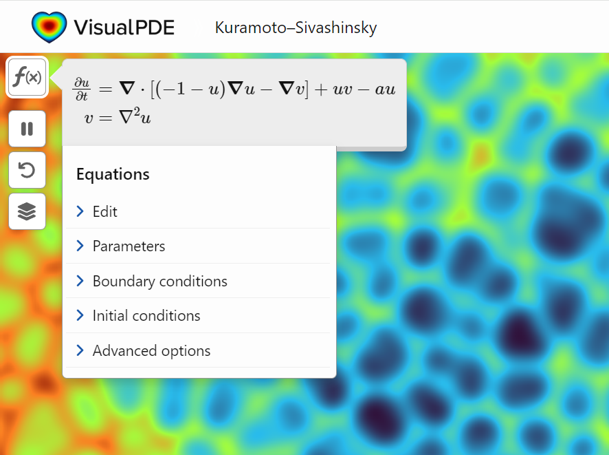
So generally I want to be using uifigures over figures. For example I really like the tab group component, which can really help with organizing large numbers of plots in a manageable way. I also really prefer the look of the progress dialog, uialert, confirm, etc. That said, I run into way more bugs using uifigures. I always get a “flicker” in the axes toolbar for example. I also have matlab getting “hung” a lot more often when using uifigures.

So in general, what is recommended? Are uifigures ever going to fully replace traditional figures? Are they going to become more and more robust? Do I need a better GPU to handle graphics better? Just looking for general guidance.

Salam Surjit
Salam Surjit
Last activity 2024-10-2,11:03

Hi everyone, I am from India ..Suggest some drone for deploying code from Matlab.
Hello :-) I am interested in reading the book "The finite element method for solid and structural mechanics" online with somebody who is also interested in studying the finite element method particularly its mathematical aspect. I enjoy discussing the book instead of reading it alone. Please if you were interested email me at: student.z.k@hotmail.com Thank you!
Image Analyst
Image Analyst
Last activity 2024-8-12

Imagine that the earth is a perfect sphere with a radius of 6371000 meters and there is a rope tightly wrapped around the equator. With one line of MATLAB code determine how much the rope will be lifted above the surface if you cut it and insert a 1 meter segment of rope into it (and then expand the whole rope back into a circle again, of course).
David
David
Last activity 2024-8-8

A library of runnable PDEs. See the equations! Modify the parameters! Visualize the resulting system in your browser! Convenient, fast, and instructive.
Swimming, diving
16%
Other water-based sport
4%
Gymnastics
20%
Other indoor arena sport
15%
track, field
24%
Other outdoor sport
21%
346 个投票
Hello, MATLAB enthusiasts! 🌟
Over the past few weeks, our community has been buzzing with insightful questions, vibrant discussions, and innovative ideas. Whether you're a seasoned expert or a curious beginner, there's something here for everyone to learn and enjoy. Let's take a moment to highlight some of the standout contributions that have sparked interest and inspired many. Dive in and see how you can join the conversation or find solutions to your own challenges!

Interesting Questions

Oluwadamilola Oke is seeking assistance with a MATLAB code that works on version r2014b but encounters errors on version r2024a. The issue seems to be related to file location or the use of specific commands like movefile. If you have experience with these versions of MATLAB, your expertise could be invaluable.
Yohay has been working on a simulation to measure particle speed and fit it to the Maxwell-Boltzmann distribution. However, the fit isn't aligning perfectly with the data. Yohay has shared the code and histogram data for community members to review and provide suggestions.
Alessandro Livi is toggling between C++ for Arduino Pico and MATLAB App Designer. They suggest an enhancement where typing // for comments in MATLAB automatically converts to %. This small feature could improve the workflow for many users who switch between programming languages.

Popular Discussions

Athanasios Paraskevopoulos has started an engaging discussion on Gabriel's Horn, a shape with infinite surface area but finite volume. The conversation delves into the mathematical intricacies and integral calculations required to understand this paradoxical shape.
Honzik has brought up an interesting topic about custom fonts for MATLAB. While popular coding fonts handle characters like 0 and O well, they often fail to distinguish between different types of brackets. Honzik suggests that MathWorks could develop a custom font optimized for MATLAB syntax to reduce coding errors.

From the Blogs

Guy Rouleau addresses a common error in Simulink models: "Derivative of state '1' in block 'X/Y/Integrator' at time 0.55 is not finite." The blog post explores various tools and methods to diagnose and resolve this issue, making it a valuable read for anyone facing similar challenges.
Guest writer Gianluca Carnielli, featured by Adam Danz, shares insights on creating time-sensitive animations using MATLAB. The article covers controlling the motion of multiple animated objects, organizing data with timetables, and simplifying animations with the retime function. This is a must-read for anyone interested in scientific animations.
Feel free to check out these fascinating contributions and join the discussions! Your input and expertise can make a significant difference in our community.
hello i found the following tools helpful to write matlab programs. copilot.microsoft.com chatgpt.com/gpts gemini.google.com and ai.meta.com. thanks a lot and best wishes.

Hi everyone,

I've recently joined a forest protection team in Greece, where we use drones for various tasks. This has sparked my interest in drone programming, and I'd like to learn more about it. Can anyone recommend any beginner-friendly courses or programs that teach drone programming?

I'm particularly interested in courses that focus on practical applications and might align with the work we do in forest protection. Any suggestions or guidance would be greatly appreciated!

Thank you!

I have picked the title but don't know which direction to take it. Looking for any and all inspiration. I took the project as it sounded interesting when reading into it, but I'm a satellite novice, and my degree is in electronics.
"What are your favorite features or functionalities in MATLAB, and how have they positively impacted your projects or research? Any tips or tricks to share?
Check out the LLMs with MATLAB project on File Exchange to access Large Language Models from MATLAB.
Along with the latest support for GPT-4o mini, you can use LLMs with MATLAB to generate images, categorize data, and provide semantic analyis.
Run it now by clicking Open in MATLAB Online, signing in, and using your API Key from OpenAI.
Gabriel's horn is a shape with the paradoxical property that it has infinite surface area, but a finite volume.
Gabriel’s horn is formed by taking the graph of with the domain and rotating it in three dimensions about the axis.
There is a standard formula for calculating the volume of this shape, for a general function .Wwe will just state that the volume of the solid between a and b is:
The surface area of the solid is given by:
One other thing we need to consider is that we are trying to find the value of these integrals between 1 and . An integral with a limit of infinity is called an improper integral and we can't evaluate it simply by plugging the value infinity into the normal equation for a definite integral. Instead, we must first calculate the definite integral up to some finite limit b and then calculate the limit of the result as b tends to :
Volume
We can calculate the horn's volume using the volume integral above, so
The total volume of this infinitely long trumpet isπ.
Surface Area
To determine the surface area, we first need the function’s derivative:
Now plug it into the surface area formula and we have:
This is an improper integral and it's hard to evaluate, but since in our interval
So, we have :
Now,we evaluate this last integral
So the surface are is infinite.
% Define the function for Gabriel's Horn
gabriels_horn = @(x) 1 ./ x;
% Create a range of x values
x = linspace(1, 40, 4000); % Increase the number of points for better accuracy
y = gabriels_horn(x);
% Create the meshgrid
theta = linspace(0, 2 * pi, 6000); % Increase theta points for a smoother surface
[X, T] = meshgrid(x, theta);
Y = gabriels_horn(X) .* cos(T);
Z = gabriels_horn(X) .* sin(T);
% Plot the surface of Gabriel's Horn
figure('Position', [200, 100, 1200, 900]);
surf(X, Y, Z, 'EdgeColor', 'none', 'FaceAlpha', 0.9);
hold on;
% Plot the central axis
plot3(x, zeros(size(x)), zeros(size(x)), 'r', 'LineWidth', 2);
% Set labels
xlabel('x');
ylabel('y');
zlabel('z');
% Adjust colormap and axis properties
colormap('gray');
shading interp; % Smooth shading
% Adjust the view
view(3);
axis tight;
grid on;
% Add formulas as text annotations
dim1 = [0.4 0.7 0.3 0.2];
annotation('textbox',dim1,'String',{'$$V = \pi \int_{1}^{a} \left( \frac{1}{x} \right)^2 dx = \pi \left( 1 - \frac{1}{a} \right)$$', ...
'', ... % Add an empty line for larger gap
'$$\lim_{a \to \infty} V = \lim_{a \to \infty} \pi \left( 1 - \frac{1}{a} \right) = \pi$$'}, ...
'Interpreter','latex','FontSize',12, 'EdgeColor','none', 'FitBoxToText', 'on');
dim2 = [0.4 0.5 0.3 0.2];
annotation('textbox',dim2,'String',{'$$A = 2\pi \int_{1}^{a} \frac{1}{x} \sqrt{1 + \left( -\frac{1}{x^2} \right)^2} dx > 2\pi \int_{1}^{a} \frac{dx}{x} = 2\pi \ln(a)$$', ...
'', ... % Add an empty line for larger gap
'$$\lim_{a \to \infty} A \geq \lim_{a \to \infty} 2\pi \ln(a) = \infty$$'}, ...
'Interpreter','latex','FontSize',12, 'EdgeColor','none', 'FitBoxToText', 'on');
% Add Gabriel's Horn label
dim3 = [0.3 0.9 0.3 0.1];
annotation('textbox',dim3,'String','Gabriel''s Horn', ...
'Interpreter','latex','FontSize',14, 'EdgeColor','none', 'HorizontalAlignment', 'center');
hold off
daspect([3.5 1 1]) % daspect([x y z])
view(-27, 15)
lightangle(-50,0)
lighting('gouraud')
The properties of this figure were first studied by Italian physicist and mathematician Evangelista Torricelli in the 17th century.
Acknowledgment
I would like to express my sincere gratitude to all those who have supported and inspired me throughout this project.
First and foremost, I would like to thank the mathematician and my esteemed colleague, Stavros Tsalapatis, for inspiring me with the fascinating subject of Gabriel's Horn.
I am also deeply thankful to Mr. @Star Strider for his invaluable assistance in completing the final code.
References:
  1. How to Find the Volume and Surface Area of Gabriel's Horn
  2. Gabriel's Horn
  3. An Understanding of a Solid with Finite Volume and Infinite Surface Area.
  4. IMPROPER INTEGRALS: GABRIEL’S HORN
  5. Gabriel’s Horn and the Painter's Paradox in Perspective
When it comes to MOS tube burnout, it is usually because it is not working in the SOA workspace, and there is also a case where the MOS tube is overcurrent.
For example, the maximum allowable current of the PMOS transistor in this circuit is 50A, and the maximum current reaches 80+ at the moment when the MOS transistor is turned on, then the current is very large.
At this time, the PMOS is over-specified, and we can see on the SOA curve that it is not working in the SOA range, which will cause the PMOS to be damaged.
So what if you choose a higher current PMOS? Of course you can, but the cost will be higher.
We can choose to adjust the peripheral resistance or capacitor to make the PMOS turn on more slowly, so that the current can be lowered.
For example, when adjusting R1, R2, and the jumper capacitance between gs, when Cgs is adjusted to 1uF, The Ids are only 40A max, which is fine in terms of current, and meets the 80% derating.
(50 amps * 0.8 = 40 amps).
Next, let’s look at the power, from the SOA curve, the opening time of the MOS tube is about 1ms, and the maximum power at this time is 280W.
The normal thermal resistance of the chip is 50°C/W, and the maximum junction temperature can be 302°F.
Assuming the ambient temperature is 77°F, then the instantaneous power that 1ms can withstand is about 357W.
The actual power of PMOS here is 280W, which does not exceed the limit, which means that it works normally in the SOA area.
Therefore, when the current impact of the MOS transistor is large at the moment of turning, the Cgs capacitance can be adjusted appropriately to make the PMOS Working in the SOA area, you can avoid the problem of MOS corruption.
Marisa
Marisa
Last activity 2024-8-26

I am trying to earn my Intro to MATLAB badge in Cody, but I cannot click the Roll the Dice! problem. It simply is not letting me click it, therefore I cannot earn my badge. Does anyone know who I should contact or what to do?