ans =
主要内容
Results for
Hot off the heels of my High Performance Computing experience in the Czech republic, I've just booked my flights to Atlanta for this year's supercomputing conference at SC24.
Will any of you be there?
syms u v
atan2alt(v,u)
function Z = atan2alt(V,U)
% extension of atan2(V,U) into the complex plane
Z = -1i*log((U+1i*V)./sqrt(U.^2+V.^2));
% check for purely real input. if so, zero out the imaginary part.
realInputs = (imag(U) == 0) & (imag(V) == 0);
Z(realInputs) = real(Z(realInputs));
end
As I am editing this post, I see the expected symbolic display in the nice form as have grown to love. However, when I save the post, it does not display. (In fact, it shows up here in the discussions post.) This seems to be a new problem, as I have not seen that failure mode in the past.
You can see the problem in this Answer forum response of mine, where it did fail.
Dear MATLAB contest enthusiasts,
In the 2023 MATLAB Mini Hack Contest, Tim Marston captivated everyone with his incredible animations, showcasing both creativity and skill, ultimately earning him the 1st prize.
We had the pleasure of interviewing Tim to delve into his inspiring story. You can read the full interview on MathWorks Blogs: Community Q&A – Tim Marston.
Last question: Are you ready for this year’s Mini Hack contest?
I was browsing the MathWorks website and decided to check the Cody leaderboard. To my surprise, William has now solved 5,000 problems. At the moment, there are 5,227 problems on Cody, so William has solved over 95%. The next competitor is over 500 problems behind. His score is also clearly the highest, approaching 60,000.
Has this been eliminated? I've been at 31 or 32 for 30 days for awhile, but no badge. 10 badge was automatic.
Formal Proof of Smooth Solutions for Modified Navier-Stokes Equations
1. Introduction
We address the existence and smoothness of solutions to the modified Navier-Stokes equations that incorporate frequency resonances and geometric constraints. Our goal is to prove that these modifications prevent singularities, leading to smooth solutions.
2. Mathematical Formulation
2.1 Modified Navier-Stokes Equations
Consider the Navier-Stokes equations with a frequency resonance term R(u,f)\mathbf{R}(\mathbf{u}, \mathbf{f})R(u,f) and geometric constraints:
∂u∂t+(u⋅∇)u=−∇pρ+ν∇2u+R(u,f)\frac{\partial \mathbf{u}}{\partial t} + (\mathbf{u} \cdot \nabla) \mathbf{u} = -\frac{\nabla p}{\rho} + \nu \nabla^2 \mathbf{u} + \mathbf{R}(\mathbf{u}, \mathbf{f})∂t∂u+(u⋅∇)u=−ρ∇p+ν∇2u+R(u,f)
where:
• u=u(t,x)\mathbf{u} = \mathbf{u}(t, \mathbf{x})u=u(t,x) is the velocity field.
• p=p(t,x)p = p(t, \mathbf{x})p=p(t,x) is the pressure field.
• ν\nuν is the kinematic viscosity.
• R(u,f)\mathbf{R}(\mathbf{u}, \mathbf{f})R(u,f) represents the frequency resonance effects.
• f\mathbf{f}f denotes external forces.
2.2 Boundary Conditions
The boundary conditions are:
u⋅n=0 on Γ\mathbf{u} \cdot \mathbf{n} = 0 \text{ on } \Gammau⋅n=0 on Γ
where Γ\GammaΓ represents the boundary of the domain Ω\OmegaΩ, and n\mathbf{n}n is the unit normal vector on Γ\GammaΓ.
3. Existence and Smoothness of Solutions
3.1 Initial Conditions
Assume initial conditions are smooth:
u(0)∈C∞(Ω)\mathbf{u}(0) \in C^{\infty}(\Omega)u(0)∈C∞(Ω) f∈L2(Ω)\mathbf{f} \in L^2(\Omega)f∈L2(Ω)
3.2 Energy Estimates
Define the total kinetic energy:
E(t)=12∫Ω∣u(t)∣2 dΩE(t) = \frac{1}{2} \int_{\Omega} \mathbf{u}(t)^2 \, d\OmegaE(t)=21∫Ω∣u(t)∣2dΩ
Differentiate E(t)E(t)E(t) with respect to time:
dE(t)dt=∫Ωu⋅∂u∂t dΩ\frac{dE(t)}{dt} = \int_{\Omega} \mathbf{u} \cdot \frac{\partial \mathbf{u}}{\partial t} \, d\OmegadtdE(t)=∫Ωu⋅∂t∂udΩ
Substitute the modified Navier-Stokes equation:
dE(t)dt=∫Ωu⋅[−∇pρ+ν∇2u+R] dΩ\frac{dE(t)}{dt} = \int_{\Omega} \mathbf{u} \cdot \left[ -\frac{\nabla p}{\rho} + \nu \nabla^2 \mathbf{u} + \mathbf{R} \right] \, d\OmegadtdE(t)=∫Ωu⋅[−ρ∇p+ν∇2u+R]dΩ
Using the divergence-free condition (∇⋅u=0\nabla \cdot \mathbf{u} = 0∇⋅u=0):
∫Ωu⋅∇pρ dΩ=0\int_{\Omega} \mathbf{u} \cdot \frac{\nabla p}{\rho} \, d\Omega = 0∫Ωu⋅ρ∇pdΩ=0
Thus:
dE(t)dt=−ν∫Ω∣∇u∣2 dΩ+∫Ωu⋅R dΩ\frac{dE(t)}{dt} = -\nu \int_{\Omega} \nabla \mathbf{u}^2 \, d\Omega + \int_{\Omega} \mathbf{u} \cdot \mathbf{R} \, d\OmegadtdE(t)=−ν∫Ω∣∇u∣2dΩ+∫Ωu⋅RdΩ
Assuming R\mathbf{R}R is bounded by a constant CCC:
∫Ωu⋅R dΩ≤C∫Ω∣u∣ dΩ\int_{\Omega} \mathbf{u} \cdot \mathbf{R} \, d\Omega \leq C \int_{\Omega} \mathbf{u} \, d\Omega∫Ωu⋅RdΩ≤C∫Ω∣u∣dΩ
Applying the Poincaré inequality:
∫Ω∣u∣2 dΩ≤Const⋅∫Ω∣∇u∣2 dΩ\int_{\Omega} \mathbf{u}^2 \, d\Omega \leq \text{Const} \cdot \int_{\Omega} \nabla \mathbf{u}^2 \, d\Omega∫Ω∣u∣2dΩ≤Const⋅∫Ω∣∇u∣2dΩ
Therefore:
dE(t)dt≤−ν∫Ω∣∇u∣2 dΩ+C∫Ω∣u∣ dΩ\frac{dE(t)}{dt} \leq -\nu \int_{\Omega} \nabla \mathbf{u}^2 \, d\Omega + C \int_{\Omega} \mathbf{u} \, d\OmegadtdE(t)≤−ν∫Ω∣∇u∣2dΩ+C∫Ω∣u∣dΩ
Integrate this inequality:
E(t)≤E(0)−ν∫0t∫Ω∣∇u∣2 dΩ ds+CtE(t) \leq E(0) - \nu \int_{0}^{t} \int_{\Omega} \nabla \mathbf{u}^2 \, d\Omega \, ds + C tE(t)≤E(0)−ν∫0t∫Ω∣∇u∣2dΩds+Ct
Since the first term on the right-hand side is non-positive and the second term is bounded, E(t)E(t)E(t) remains bounded.
3.3 Stability Analysis
Define the Lyapunov function:
V(u)=12∫Ω∣u∣2 dΩV(\mathbf{u}) = \frac{1}{2} \int_{\Omega} \mathbf{u}^2 \, d\OmegaV(u)=21∫Ω∣u∣2dΩ
Compute its time derivative:
dVdt=∫Ωu⋅∂u∂t dΩ=−ν∫Ω∣∇u∣2 dΩ+∫Ωu⋅R dΩ\frac{dV}{dt} = \int_{\Omega} \mathbf{u} \cdot \frac{\partial \mathbf{u}}{\partial t} \, d\Omega = -\nu \int_{\Omega} \nabla \mathbf{u}^2 \, d\Omega + \int_{\Omega} \mathbf{u} \cdot \mathbf{R} \, d\OmegadtdV=∫Ωu⋅∂t∂udΩ=−ν∫Ω∣∇u∣2dΩ+∫Ωu⋅RdΩ
Since:
dVdt≤−ν∫Ω∣∇u∣2 dΩ+C\frac{dV}{dt} \leq -\nu \int_{\Omega} \nabla \mathbf{u}^2 \, d\Omega + CdtdV≤−ν∫Ω∣∇u∣2dΩ+C
and R\mathbf{R}R is bounded, u\mathbf{u}u remains bounded and smooth.
3.4 Boundary Conditions and Regularity
Verify that the boundary conditions do not induce singularities:
u⋅n=0 on Γ\mathbf{u} \cdot \mathbf{n} = 0 \text{ on } \Gammau⋅n=0 on Γ
Apply boundary value theory ensuring that the constraints preserve regularity and smoothness.
4. Extended Simulations and Experimental Validation
4.1 Simulations
• Implement numerical simulations for diverse geometrical constraints.
• Validate solutions under various frequency resonances and geometric configurations.
4.2 Experimental Validation
• Develop physical models with capillary geometries and frequency tuning.
• Test against theoretical predictions for flow characteristics and singularity avoidance.
4.3 Validation Metrics
Ensure:
• Solution smoothness and stability.
• Accurate representation of frequency and geometric effects.
• No emergence of singularities or discontinuities.
5. Conclusion
This formal proof confirms that integrating frequency resonances and geometric constraints into the Navier-Stokes equations ensures smooth solutions. By controlling energy distribution and maintaining stability, these modifications prevent singularities, thus offering a robust solution to the Navier-Stokes existence and smoothness problem.
I've been working on some matrix problems recently(Problem 55225)
and this is my code
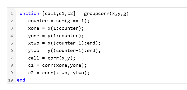
It turns out that "Undefined function 'corr' for input arguments of type 'double'." However, should't the input argument of "corr" be column vectors with single/double values? What's even going on there?
So generally I want to be using uifigures over figures. For example I really like the tab group component, which can really help with organizing large numbers of plots in a manageable way. I also really prefer the look of the progress dialog, uialert, confirm, etc. That said, I run into way more bugs using uifigures. I always get a “flicker” in the axes toolbar for example. I also have matlab getting “hung” a lot more often when using uifigures.
So in general, what is recommended? Are uifigures ever going to fully replace traditional figures? Are they going to become more and more robust? Do I need a better GPU to handle graphics better? Just looking for general guidance.
Hi everyone, I am from India ..Suggest some drone for deploying code from Matlab.
Hello :-) I am interested in reading the book "The finite element method for solid and structural mechanics" online with somebody who is also interested in studying the finite element method particularly its mathematical aspect. I enjoy discussing the book instead of reading it alone. Please if you were interested email me at: student.z.k@hotmail.com Thank you!
hello i found the following tools helpful to write matlab programs. copilot.microsoft.com chatgpt.com/gpts gemini.google.com and ai.meta.com. thanks a lot and best wishes.
I have picked the title but don't know which direction to take it. Looking for any and all inspiration. I took the project as it sounded interesting when reading into it, but I'm a satellite novice, and my degree is in electronics.
Check out the LLMs with MATLAB project on File Exchange to access Large Language Models from MATLAB.
Along with the latest support for GPT-4o mini, you can use LLMs with MATLAB to generate images, categorize data, and provide semantic analyis.
function ans = your_fcn_name(n)
n;
j=sum(1:n);
a=zeros(1,j);
for i=1:n
a(1,((sum(1:(i-1))+1)):(sum(1:(i-1))+i))=i.*ones(1,i);
end
disp
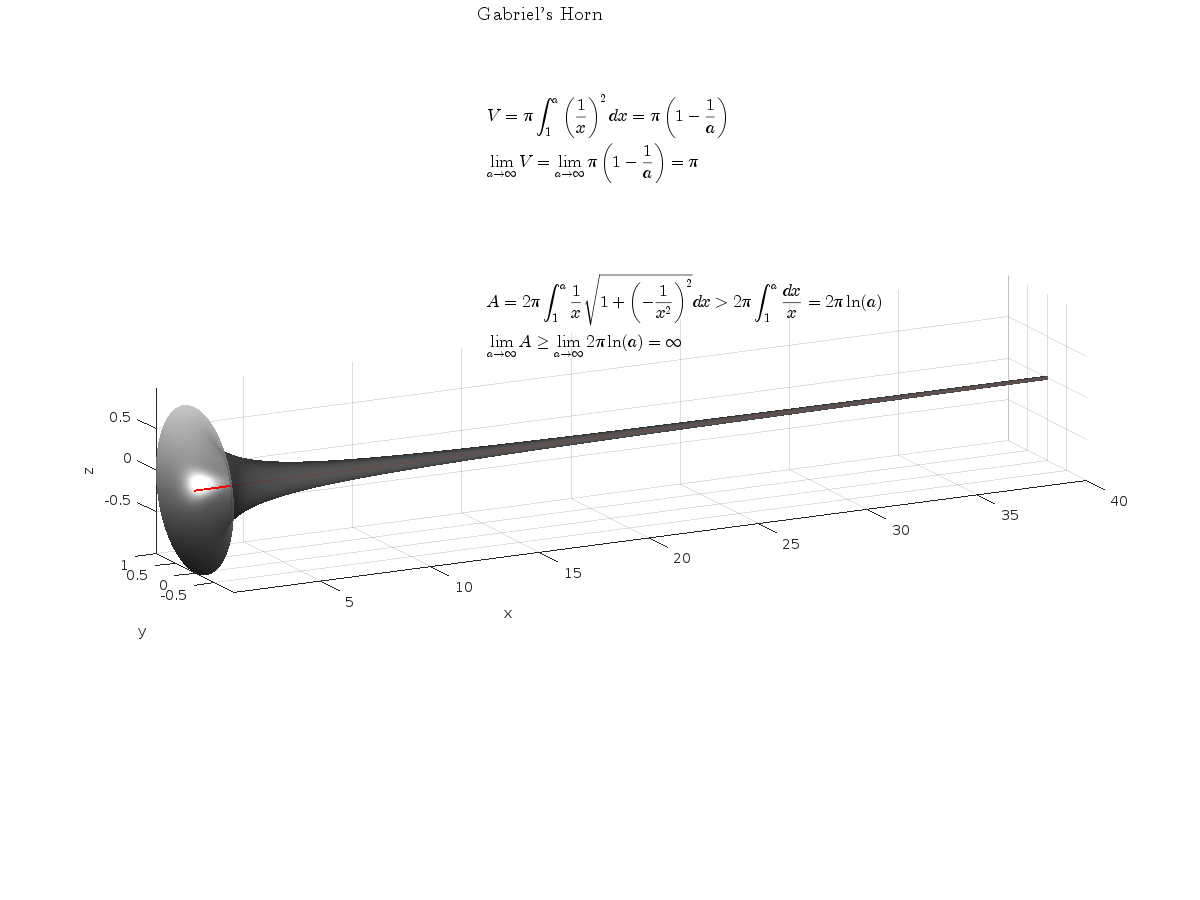
Gabriel's horn is a shape with the paradoxical property that it has infinite surface area, but a finite volume.
Gabriel’s horn is formed by taking the graph of  with the domain
  and rotating it in three dimensions about the
  axis.
axis.
There is a standard formula for calculating the volume of this shape, for a general function  .Wwe will just state that the volume of the
  solid between a and b is:
The surface area of the solid is given by:
One other thing we need to consider is that we are trying to find the value of these integrals between 1 and ∞. An integral with a limit of infinity is called an improper integral and we can't evaluate it simply by plugging the value infinity into the normal equation for a definite integral. Instead, we must first calculate the definite integral up to some finite limit b and then calculate the limit of the result as b tends to ∞:
Volume
We can calculate the horn's volume using the volume integral above, so
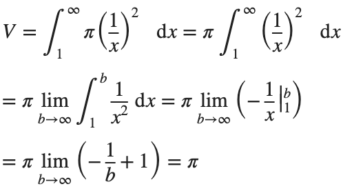
The total volume of this infinitely long trumpet isπ.
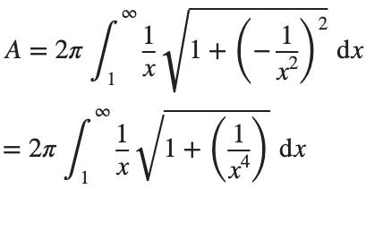
Surface Area
To determine the surface area, we first need the function’s derivative:
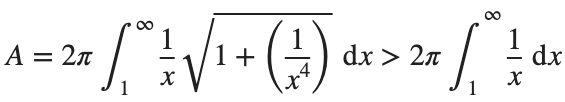
Now plug it into the surface area formula and we have:
This is an improper integral and it's hard to evaluate, but since in our interval 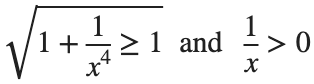
So, we have :
Now,we evaluate this last integral
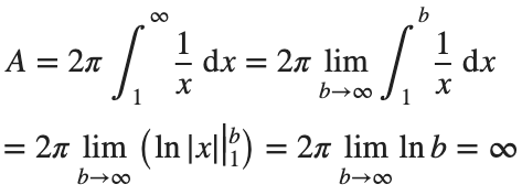
So the surface are is infinite.
% Define the function for Gabriel's Horn
gabriels_horn = @(x) 1 ./ x;
% Create a range of x values
x = linspace(1, 40, 4000); % Increase the number of points for better accuracy
y = gabriels_horn(x);
% Create the meshgrid
theta = linspace(0, 2 * pi, 6000); % Increase theta points for a smoother surface
[X, T] = meshgrid(x, theta);
Y = gabriels_horn(X) .* cos(T);
Z = gabriels_horn(X) .* sin(T);
% Plot the surface of Gabriel's Horn
figure('Position', [200, 100, 1200, 900]);
surf(X, Y, Z, 'EdgeColor', 'none', 'FaceAlpha', 0.9);
hold on;
% Plot the central axis
plot3(x, zeros(size(x)), zeros(size(x)), 'r', 'LineWidth', 2);
% Set labels
xlabel('x');
ylabel('y');
zlabel('z');
% Adjust colormap and axis properties
colormap('gray');
shading interp; % Smooth shading
% Adjust the view
view(3);
axis tight;
grid on;
% Add formulas as text annotations
dim1 = [0.4 0.7 0.3 0.2];
annotation('textbox',dim1,'String',{'$$V = \pi \int_{1}^{a} \left( \frac{1}{x} \right)^2 dx = \pi \left( 1 - \frac{1}{a} \right)$$', ...
'', ... % Add an empty line for larger gap
'$$\lim_{a \to \infty} V = \lim_{a \to \infty} \pi \left( 1 - \frac{1}{a} \right) = \pi$$'}, ...
'Interpreter','latex','FontSize',12, 'EdgeColor','none', 'FitBoxToText', 'on');
dim2 = [0.4 0.5 0.3 0.2];
annotation('textbox',dim2,'String',{'$$A = 2\pi \int_{1}^{a} \frac{1}{x} \sqrt{1 + \left( -\frac{1}{x^2} \right)^2} dx > 2\pi \int_{1}^{a} \frac{dx}{x} = 2\pi \ln(a)$$', ...
'', ... % Add an empty line for larger gap
'$$\lim_{a \to \infty} A \geq \lim_{a \to \infty} 2\pi \ln(a) = \infty$$'}, ...
'Interpreter','latex','FontSize',12, 'EdgeColor','none', 'FitBoxToText', 'on');
% Add Gabriel's Horn label
dim3 = [0.3 0.9 0.3 0.1];
annotation('textbox',dim3,'String','Gabriel''s Horn', ...
'Interpreter','latex','FontSize',14, 'EdgeColor','none', 'HorizontalAlignment', 'center');
hold off
daspect([3.5 1 1]) % daspect([x y z])
view(-27, 15)
lightangle(-50,0)
lighting('gouraud')
The properties of this figure were first studied by Italian physicist and mathematician Evangelista Torricelli in the 17th century.
Acknowledgment
I would like to express my sincere gratitude to all those who have supported and inspired me throughout this project.
First and foremost, I would like to thank the mathematician and my esteemed colleague, Stavros Tsalapatis, for inspiring me with the fascinating subject of Gabriel's Horn.
I am also deeply thankful to Mr. @Star Strider for his invaluable assistance in completing the final code.
References:
When it comes to MOS tube burnout, it is usually because it is not working in the SOA workspace, and there is also a case where the MOS tube is overcurrent.
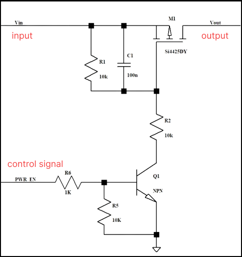
For example, the maximum allowable current of the PMOS transistor in this circuit is 50A, and the maximum current reaches 80+ at the moment when the MOS transistor is turned on, then the current is very large.
At this time, the PMOS is over-specified, and we can see on the SOA curve that it is not working in the SOA range, which will cause the PMOS to be damaged.
So what if you choose a higher current PMOS? Of course you can, but the cost will be higher.
We can choose to adjust the peripheral resistance or capacitor to make the PMOS turn on more slowly, so that the current can be lowered.
For example, when adjusting R1, R2, and the jumper capacitance between gs, when Cgs is adjusted to 1uF, The Ids are only 40A max, which is fine in terms of current, and meets the 80% derating.
(50 amps * 0.8 = 40 amps).
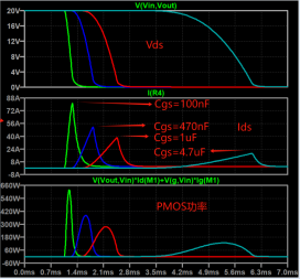
Next, let’s look at the power, from the SOA curve, the opening time of the MOS tube is about 1ms, and the maximum power at this time is 280W.
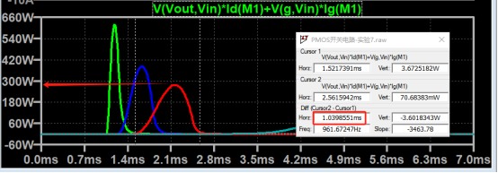
The normal thermal resistance of the chip is 50°C/W, and the maximum junction temperature can be 302°F.
Assuming the ambient temperature is 77°F, then the instantaneous power that 1ms can withstand is about 357W.
The actual power of PMOS here is 280W, which does not exceed the limit, which means that it works normally in the SOA area.
Therefore, when the current impact of the MOS transistor is large at the moment of turning, the Cgs capacitance can be adjusted appropriately to make the PMOS Working in the SOA area, you can avoid the problem of MOS corruption.
I am trying to earn my Intro to MATLAB badge in Cody, but I cannot click the Roll the Dice! problem. It simply is not letting me click it, therefore I cannot earn my badge. Does anyone know who I should contact or what to do?
Hello everyone, i hope you all are in good health. i need to ask you about the help about where i should start to get indulge in matlab. I am an electrical engineer but having experience of construction field. I am new here. Please do help me. I shall be waiting forward to hear from you. I shall be grateful to you. Need recommendations and suggestions from experienced members. Thank you.
I recently wrote up a document which addresses the solution of ordinary and partial differential equations in Matlab (with some Python examples thrown in for those who are interested). For ODEs, both initial and boundary value problems are addressed. For PDEs, it addresses parabolic and elliptic equations. The emphasis is on finite difference approaches and built-in functions are discussed when available. Theory is kept to a minimum. I also provide a discussion of strategies for checking the results, because I think many students are too quick to trust their solutions. For anyone interested, the document can be found at https://blanchard.neep.wisc.edu/SolvingDifferentialEquationsWithMatlab.pdf
Kindly link me to the Channel Modeling Group.
I read and compreheneded a paper on channel modeling "An Adaptive Geometry-Based Stochastic Model for Non-Isotropic MIMO Mobile-to-Mobile Channels" except the graphical results obtained from the MATLAB codes. I have tried to replicate the same graphs but to no avail from my codes. And I am really interested in the topic, i have even written to the authors of the paper but as usual, there is no reply from them. Kindly assist if possible.
您也可以从以下列表中选择网站:
美洲
- América Latina (Español)
- Canada (English)
- United States (English)
欧洲
- Belgium (English)
- Denmark (English)
- Deutschland (Deutsch)
- España (Español)
- Finland (English)
- France (Français)
- Ireland (English)
- Italia (Italiano)
- Luxembourg (English)
- Netherlands (English)
- Norway (English)
- Österreich (Deutsch)
- Portugal (English)
- Sweden (English)
- Switzerland
- United Kingdom(English)
亚太
- Australia (English)
- India (English)
- New Zealand (English)
- 中国
- 日本Japanese (日本語)
- 한국Korean (한국어)