ans = 
主要内容
搜索
Hi! My name is Mike McLernon, and I’m a product marketing engineer with MathWorks. In my role, I look at the trends ongoing in the wireless industry, across lots of different standards (think 5G, WLAN, SatCom, Bluetooth, etc.), and I seek to shape and guide the software that MathWorks builds to respond to these trends. That’s all about communicating within the Mathworks organization, but every so often it’s worth communicating these trends to our audience in the world at large. Many of the people reading this are engineers (or engineers at heart), and we all want to know what’s happening in the geek world around us. I think that now is one of these times to communicate an important milestone. So, without further ado . . .
Bluetooth 6.0 is here! Announced in September by the Bluetooth Special Interest Group (SIG), it’s making more advances in its quest to create a “world without wires”. A few of the salient features in Bluetooth 6.0 are:
- Channel sounding (for accurate distance measurements)
- Decision-based advertising filtering (for more efficient channel scanning)
- Monitoring advertisers (for improved energy efficiency when devices come into and go out of range)
- Frame space updates (for both higher throughput and better coexistence management)
Bluetooth 6.0 includes other features as well, but the SIG has put special promotional emphasis on channel sounding (CS), which once upon a time was called High Accuracy Distance Measurement (HADM). The SIG has said that CS is a step towards true distance awareness, and 10 cm ranging accuracy. I think their emphasis is in exactly the right place, so let’s learn more about this technology and how it is used.
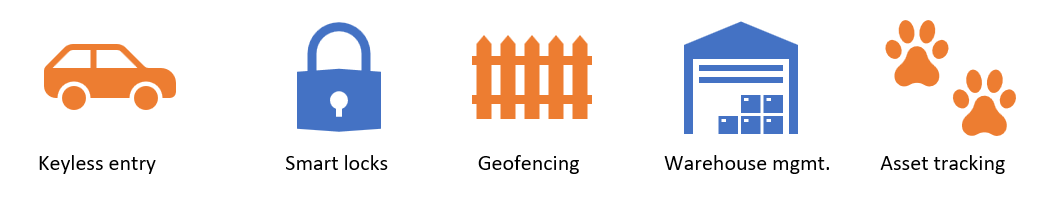
CS can be used for the following use cases:
- Keyless vehicle entry, performed by communication between a key fob or phone and the car’s anchor points
- Smart locks, to permit access only when an authorized device is within a designated proximity to the locks
- Geofencing, to limit access to designated areas
- Warehouse management, to monitor inventory and manage logistics
- Asset tracking for virtually any object of interest
In the past, Bluetooth devices would use a received signal strength indicator (RSSI) measurement to infer the distance between two of them. They would assume a free space path loss on the link, and use a straightforward equation to estimate distance:
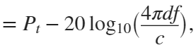 where
whereSo in this method, 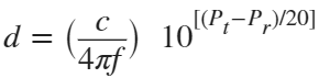 . But if the signal suffers more loss from multipath or shadowing, then the distance would be overestimated. Something better needed to be found.
. But if the signal suffers more loss from multipath or shadowing, then the distance would be overestimated. Something better needed to be found.Bluetooth 6.0 introduces not one, but two ways to accurately measure distance:
- Round-trip time (RTT) measurement
- Phase-based ranging (PBR) measurement
The RTT measurement method uses the fact that the Bluetooth signal time of flight (TOF) between two devices is half the RTT. It can then accurately compute the distance d as
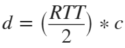 , where c is again the speed of light. This method requires accurate measurements of the time of departure (TOD) of the outbound signal from device 1 (the Initiator), time of arrival (TOA) of the outbound signal to device 2 (the Reflector), TOD of the return signal from device 2, and TOA of the return signal to device 1. The diagram below shows the signal paths and the times.
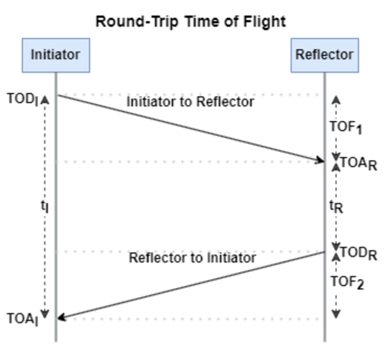
If you want to see how you can use MATLAB to simulate the RTT method, take a look at Estimate Distance Between Bluetooth LE Devices by Using Channel Sounding and Round-Trip Timing.
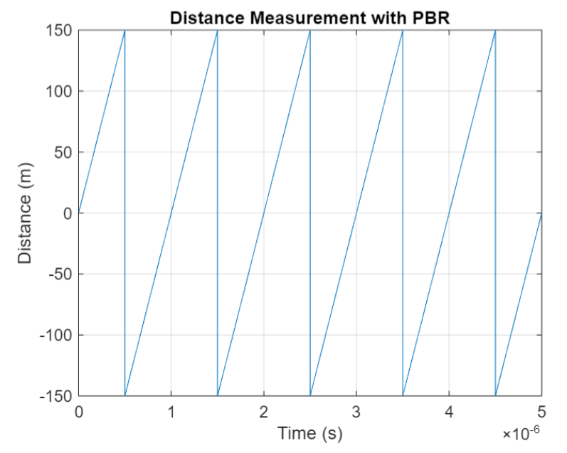
The PBR method uses two Bluetooth signals of different frequencies to measure distance. These signals are simply tones – sine waves. Without going through the derivation, PBR calculates distance d as
The mod() operation is needed to eliminate ambiguities in the distance calculation and the final division by two is to convert a round trip distance to a one-way distance. Because a given phase difference value can hold true for an infinite number of distance values, the mod() operation chooses the smallest distance that satisfies the equation. Also, these tones can be as close as 1 MHz apart. In that case, the maximum resolvable distance measurement is about 150 m. The plot below shows that ambiguity and repetition in distance measurement.
If you want to see how you can use MATLAB to simulate the PBR method, take a look at Estimate Distance Between Bluetooth LE Devices by Using Channel Sounding and Phase-Based Ranging.
Bluetooth 6.0 outlines RTT and PBR distance measurement methods, but CS does not mandate a specific algorithm for calculating distance estimates. This flexibility allows device manufacturers to tailor solutions to various use cases, balancing computational complexity with required accuracy and adapting to different radio environments. Examples include simple phase difference calculations and FFT-based methods.
Although Bluetooth 6.0 is now out, it is far from a finished version. The SIG is actively working through the ratification process for two major extensions:
- High Data Throughput, up to 8 Mbps
- 5 and 6 GHz operation
See the last few minutes of this video from the SIG to learn more about these exciting future developments. And if you want to see more Bluetooth blogs, give a review of this one! Finally, if you have specific Bluetooth questions, give me a shout and let’s start a discussion!
So I made this.
clear
close all
clc
% inspired from: https://www.youtube.com/watch?v=3CuUmy7jX6k
%% user parameters
h = 768;
w = 1024;
N_snowflakes = 50;
%% set figure window
figure(NumberTitle="off", ...
name='Mat-snowfalling-lab (right click to stop)', ...
MenuBar="none")
ax = gca;
ax.XAxisLocation = 'origin';
ax.YAxisLocation = 'origin';
axis equal
axis([0, w, 0, h])
ax.Color = 'k';
ax.XAxis.Visible = 'off';
ax.YAxis.Visible = 'off';
ax.Position = [0, 0, 1, 1];
%% first snowflake
ht = gobjects(1, 1);
for i=1:length(ht)
ht(i) = hgtransform();
ht(i).UserData = snowflake_factory(h, w);
ht(i).Matrix(2, 4) = ht(i).UserData.y;
ht(i).Matrix(1, 4) = ht(i).UserData.x;
im = imagesc(ht(i), ht(i).UserData.img);
im.AlphaData = ht(i).UserData.alpha;
colormap gray
end
%% falling snowflake
tic;
while true
% add a snowflake every 0.3 seconds
if toc > 0.3
if length(ht) < N_snowflakes
ht = [ht; hgtransform()];
ht(end).UserData = snowflake_factory(h, w);
ht(end).Matrix(2, 4) = ht(end).UserData.y;
ht(end).Matrix(1, 4) = ht(end).UserData.x;
im = imagesc(ht(end), ht(end).UserData.img);
im.AlphaData = ht(end).UserData.alpha;
colormap gray
end
tic;
end
ax.CLim = [0, 0.0005]; % prevent from auto clim
% move snowflakes
for i = 1:length(ht)
ht(i).Matrix(2, 4) = ht(i).Matrix(2, 4) + ht(i).UserData.velocity;
end
if strcmp(get(gcf, 'SelectionType'), 'alt')
set(gcf, 'SelectionType', 'normal')
break
end
drawnow
% delete the snowflakes outside the window
for i = length(ht):-1:1
if ht(i).Matrix(2, 4) < -length(ht(i).Children.CData)
delete(ht(i))
ht(i) = [];
end
end
end
%% snowflake factory
function snowflake = snowflake_factory(h, w)
radius = round(rand*h/3 + 10);
sigma = radius/6;
snowflake.velocity = -rand*0.5 - 0.1;
snowflake.x = rand*w;
snowflake.y = h - radius/3;
snowflake.img = fspecial('gaussian', [radius, radius], sigma);
snowflake.alpha = snowflake.img/max(max(snowflake.img));
end
It would be nice to have a function to shade between two curves. This is a common question asked on Answers and there are some File Exchange entries on it but it's such a common thing to want to do I think there should be a built in function for it. I'm thinking of something like
plotsWithShading(x1, y1, 'r-', x2, y2, 'b-', 'ShadingColor', [.7, .5, .3], 'Opacity', 0.5);
So we can specify the coordinates of the two curves, and the shading color to be used, and its opacity, and it would shade the region between the two curves where the x ranges overlap. Other options should also be accepted, like line with, line style, markers or not, etc. Perhaps all those options could be put into a structure as fields, like
plotsWithShading(x1, y1, options1, x2, y2, options2, 'ShadingColor', [.7, .5, .3], 'Opacity', 0.5);
the shading options could also (optionally) be a structure. I know it can be done with a series of other functions like patch or fill, but it's kind of tricky and not obvious as we can see from the number of questions about how to do it.
Does anyone else think this would be a convenient function to add?
In the past two years, large language models have brought us significant changes, leading to the emergence of programming tools such as GitHub Copilot, Tabnine, Kite, CodeGPT, Replit, Cursor, and many others. Most of these tools support code writing by providing auto-completion, prompts, and suggestions, and they can be easily integrated with various IDEs.
As far as I know, aside from the MATLAB-VSCode/MatGPT plugin, MATLAB lacks such AI assistant plugins for its native MATLAB-Desktop, although it can leverage other third-party plugins for intelligent programming assistance. There is hope for a native tool of this kind to be built-in.
Hi everyone, I wrote several fancy functions that may help your coding experience, since they are in very early developing stage, I will be thankful if anyone could try them and give some feedbacks. Currently I have following:
- fstr: a Python f-string like expression
- printf: an easy to use fprintf function, accepts multiple arguments with seperator, end string control.
I will bring more functions or packages like logger when I am available.
The code is open sourced at GitHub with simple examples: https://github.com/bentrainer/MMGA
MATLAB Comprehensive commands list:
- clc - clears command window, workspace not affected
- clear - clears all variables from workspace, all variable values are lost
- diary - records into a file almost everything that appears in command window.
- exit - exits the MATLAB session
- who - prints all variables in the workspace
- whos - prints all variables in current workspace, with additional information.
Ch. 2 - Basics:
- Mathematical constants: pi, i, j, Inf, Nan, realmin, realmax
- Precedence rules: (), ^, negation, */, +-, left-to-right
- and, or, not, xor
- exp - exponential
- log - natural logarithm
- log10 - common logarithm (base 10)
- sqrt (square root)
- fprintf("final amount is %f units.", amt);
- can have: %f, %d, %i, %c, %s
- %f - fixed-point notation
- %e - scientific notation with lowercase e
- disp - outputs to a command window
- % - fieldWith.precision convChar
- MyArray = [startValue : IncrementingValue : terminatingValue]
Linspace
linspace(xStart, xStop, numPoints)
% xStart: Starting value
% xStop: Stop value
% numPoints: Number of linear-spaced points, including xStart and xStop
% Outputs a row array with the resulting values
Logspace
logspace(powerStart, powerStop, numPoints)
% powerStart: Starting value 10^powerStart
% powerStop: Stop value 10^powerStop
% numPoints: Number of logarithmic spaced points, including 10^powerStart and 10^powerStop
% Outputs a row array with the resulting values
- Transpose an array with []'
Element-Wise Operations
rowVecA = [1, 4, 5, 2];
rowVecB = [1, 3, 0, 4];
sumEx = rowVecA + rowVecB % Element-wise addition
diffEx = rowVecA - rowVecB % Element-wise subtraction
dotMul = rowVecA .* rowVecB % Element-wise multiplication
dotDiv = rowVecA ./ rowVecB % Element-wise division
dotPow = rowVecA .^ rowVecB % Element-wise exponentiation
- isinf(A) - check if the array elements are infinity
- isnan(A)
Rounding Functions
- ceil(x) - rounds each element of x to nearest integer >= to element
- floor(x) - rounds each element of x to nearest integer <= to element
- fix(x) - rounds each element of x to nearest integer towards 0
- round(x) - rounds each element of x to nearest integer. if round(x, N), rounds N digits to the right of the decimal point.
- rem(dividend, divisor) - produces a result that is either 0 or has the same sign as the dividen.
- mod(dividend, divisor) - produces a result that is either 0 or same result as divisor.
- Ex: 12/2, 12 is dividend, 2 is divisor
- sum(inputArray) - sums all entires in array
Complex Number Functions
- abs(z) - absolute value, is magnitude of complex number (phasor form r*exp(j0)
- angle(z) - phase angle, corresponds to 0 in r*exp(j0)
- complex(a,b) - creates complex number z = a + jb
- conj(z) - given complex conjugate a - jb
- real(z) - extracts real part from z
- imag(z) - extracts imaginary part from z
- unwrap(z) - removes the modulus 2pi from an array of phase angles.
Statistics Functions
- mean(xAr) - arithmetic mean calculated.
- std(xAr) - calculated standard deviation
- median(xAr) - calculated the median of a list of numbers
- mode(xAr) - calculates the mode, value that appears most often
- max(xAr)
- min(xAr)
- If using &&, this means that if first false, don't bother evaluating second
Random Number Functions
- rand(numRand, 1) - creates column array
- rand(1, numRand) - creates row array, both with numRand elements, between 0 and 1
- randi(maxRandVal, numRan, 1) - creates a column array, with numRand elements, between 1 and maxRandValue.
- randn(numRand, 1) - creates a column array with normally distributed values.
- Ex: 10 * rand(1, 3) + 6
- "10*rand(1, 3)" produces a row array with 3 random numbers between 0 and 10. Adding 6 to each element results in random values between 6 and 16.
- randi(20, 1, 5)
- Generates 5 (last argument) random integers between 1 (second argument) and 20 (first argument). The arguments 1 and 5 specify a 1 × 5 row array is returned.
Discrete Integer Mathematics
- primes(maxVal) - returns prime numbers less than or equal to maxVal
- isprime(inputNums) - returns a logical array, indicating whether each element is a prime number
- factor(intVal) - returns the prime factors of a number
- gcd(aVals, bVals) - largest integer that divides both a and b without a remainder
- lcm(aVals, bVals) - smallest positive integer that is divisible by both a and b
- factorial(intVals) - returns the factorial
- perms(intVals) - returns all the permutations of the elements int he array intVals in a 2D array pMat.
- randperm(maxVal)
- nchoosek(n, k)
- binopdf(x, n, p)
Concatenation
- cat, vertcat, horzcat
- Flattening an array, becomes vertical: sampleList = sampleArray ( : )
Dimensional Properties of Arrays
- nLargest = length(inArray) - number of elements along largest dimension
- nDim = ndims(inArray)
- nArrElement = numel(inArray) - nuber of array elements
- [nRow, nCol] = size(inArray) - returns the number of rows and columns on array. use (inArray, 1) if only row, (inArray, 2) if only column needed
- aZero = zeros(m, n) - creates an m by n array with all elements 0
- aOnes = ones(m, n) - creates an m by n array with all elements set to 1
- aEye = eye(m, n) - creates an m by n array with main diagonal ones
- aDiag = diag(vector) - returns square array, with diagonal the same, 0s elsewhere.
- outFlipLR = fliplr(A) - Flips array left to right.
- outFlipUD = flipud(A) - Flips array upside down.
- outRot90 = rot90(A) - Rotates array by 90 degrees counter clockwise around element at index (1,1).
- outTril = tril(A) - Returns the lower triangular part of an array.
- outTriU = triu(A) - Returns the upper triangular part of an array.
- arrayOut = repmat(subarrayIn, mRow, nCol), creates a large array by replicating a smaller array, with mRow x nCol tiling of copies of subarrayIn
- reshapeOut - reshape(arrayIn, numRow, numCol) - returns array with modifid dimensions. Product must equal to arrayIn of numRow and numCol.
- outLin = find(inputAr) - locates all nonzero elements of inputAr and returns linear indices of these elements in outLin.
- [sortOut, sortIndices] = sort(inArray) - sorts elements in ascending order, results result in sortOut. specify 'descend' if you want descending order. sortIndices hold the sorted indices of the array elements, which are row indices of the elements of sortOut in the original array
- [sortOut, sortIndices] = sortrows(inArray, colRef) - sorts array based on values in column colRef while keeping the rows together. Bases on first column by default.
- isequal(inArray1, inarray2, ..., inArrayN)
- isequaln(inArray1, inarray2, ..., inarrayn)
- arrayChar = ischar(inArray) - ischar tests if the input is a character array.
- arrayLogical = islogical(inArray) - islogical tests for logical array.
- arrayNumeric = isnumeric(inArray) - isnumeric tests for numeric array.
- arrayInteger = isinteger(inArray) - isinteger tests whether the input is integer type (Ex: uint8, uint16, ...)
- arrayFloat = isfloat(inArray) - isfloat tests for floating-point array.
- arrayReal= isreal(inArray) - isreal tests for real array.
- objIsa = isa(obj,ClassName) - isa determines whether input obj is an object of specified class ClassName.
- arrayScalar = isscalar(inArray) - isscalar tests for scalar type.
- arrayVector = isvector(inArray) - isvector tests for a vector (a 1D row or column array).
- arrayColumn = iscolumn(inArray) - iscolumn tests for column 1D arrays.
- arrayMatrix = ismatrix(inArray) - ismatrix returns true for a scalar or array up to 2D, but false for an array of more than 2 dimensions.
- arrayEmpty = isempty(inArray) - isempty tests whether inArray is empty.
- primeArray = isprime(inArray) - isprime returns a logical array primeArray, of the same size as inArray. The value at primeArray(index) is true when inArray(index) is a prime number. Otherwise, the values are false.
- finiteArray = isfinite(inArray) - isfinite returns a logical array finiteArray, of the same size as inArray. The value at finiteArray(index) is true when inArray(index) is finite. Otherwise, the values are false.
- infiniteArray = isinf(inArray) - isinf returns a logical array infiniteArray, of the same size as inArray. The value at infiniteArray(index) is true when inArray(index) is infinite. Otherwise, the values are false.
- nanArray = isnan(inArray) - isnan returns a logical array nanArray, of the same size as inArray. The value at nanArray(index) is true when inArray(index) is NaN. Otherwise, the values are false.
- allNonzero = all(inArray) - all identifies whether all array elements are non-zero (true). Instead of testing elements along the columns, all(inArray, 2) tests along the rows. all(inArray,1) is equivalent to all(inArray).
- anyNonzero = any(inArray) - any identifies whether any array elements are non-zero (true), and false otherwise. Instead of testing elements along the columns, any(inArray, 2) tests along the rows. any(inArray,1) is equivalent to any(inArray).
- logicArray = ismember(inArraySet,areElementsMember) - ismember returns a logical array logicArray the same size as inArraySet. The values at logicArray(i) are true where the elements of the first array inArraySet are found in the second array areElementsMember. Otherwise, the values are false. Similar values found by ismember can be extracted with inArraySet(logicArray).
- any(x) - Returns true if x is nonzero; otherwise, returns false.
- isnan(x) - Returns true if x is NaN (Not-a-Number); otherwise, returns false.
- isfinite(x) - Returns true if x is finite; otherwise, returns false. Ex: isfinite(Inf) is false, and isfinite(10) is true.
- isinf(x) - Returns true if x is +Inf or -Inf; otherwise, returns false.
Relational Operators
a & b, and(a, b)
a | b, or(a, b)
~a, not(a)
xor(a, b)
- fctName = @(arglist) expression - anonymous function
- nargin - keyword returns the number of input arguments passed to the function.
Looping
while condition
% code
end
for index = startVal:endVal
% code
end
- continue: Skips the rest of the current loop iteration and begins the next iteration.
- break: Exits a loop before it has finished all iterations.
switch expression
case value1
% code
case value2
% code
otherwise
% code
end
Comprehensive Overview (may repeat)
Built in functions/constants
abs(x) - absolute value
pi - 3.1415...
inf - ∞
eps - floating point accuracy 1e6 106
sum(x) - sums elements in x
cumsum(x) - Cumulative sum
prod - Product of array elements cumprod(x) cumulative product
diff - Difference of elements round/ceil/fix/floor Standard functions..
*Standard functions: sqrt, log, exp, max, min, Bessel *Factorial(x) is only precise for x < 21
Variable Generation
j:k - row vector
j:i:k - row vector incrementing by i
linspace(a,b,n) - n points linearly spaced and including a and b
NaN(a,b) - axb matrix of NaN values
ones(a,b) - axb matrix with all 1 values
zeros(a,b) - axb matrix with all 0 values
meshgrid(x,y) - 2d grid of x and y vectors
global x
Ch. 11 - Custom Functions
function [ outputArgs ] = MainFunctionName (inputArgs)
% statements go here
end
function [ outputArgs ] = LocalFunctionName (inputArgs)
% statements go here
end
- You are allowed to have nested functions in MATLAB
Anonymous Function:
- fctName = @(argList) expression
- Ex: RaisedCos = @(angle) (cosd(angle))^2;
- global variables - can be accessed from anywhere in the file
- Persistent variables
- persistent variable - only known to function where it was declared, maintains value between calls to function.
- Recursion - base case, decreasing case, ending case
- nargin - evaluates to the number of arguments the function was called with
Ch. 12 - Plotting
- plot(xArray, yArray)
- refer to help plot for more extensive documentation, chapter 12 only briefly covers plotting
plot - Line plot
yyaxis - Enables plotting with y-axes on both left and right sides
loglog - Line plot with logarithmic x and y axes
semilogy - Line plot with linear x and logarithmic y axes
semilogx - Line plot with logarithmic x and linear y axes
stairs - Stairstep graph
axis - sets the aspect ratio of x and y axes, ticks etc.
grid - adds a grid to the plot
gtext - allows positioning of text with the mouse
text - allows placing text at specified coordinates of the plot
xlabel labels the x-axis
ylabel labels the y-axis
title sets the graph title
figure(n) makes figure number n the current figure
hold on allows multiple plots to be superimposed on the same axes
hold off releases hold on current plot and allows a new graph to be drawn
close(n) closes figure number n
subplot(a, b, c) creates an a x b matrix of plots with c the current figure
orient specifies the orientation of a figure
Animated plot example:
for j = 1:360
pause(0.02)
plot3(x(j),y(j),z(j),'O')
axis([minx maxx miny maxy minz maxz]);
hold on;
end
Ch. 13 - Strings
stringArray = string(inputArray) - converts the input array inputArray to a string array
number = strLength(stringIn) - returns the number of characters in the input string
stringArray = strings(n, m) - returns an n-by-m array of strings with no characters,
- doing strings(sz) returns an array of strings with no characters, where sz defines the size.
charVec1 = char(stringScalar) char(stringScalar) converts the string scalar stringScalar into a character vector charVec1.
charVec2 = char(numericArray) char(numericArray) converts the numeric array numericArray into a character vector charVec2 corresponding to the Unicode transformation format 16 (UTF-16) code.
stringOut = string1 + string2 - combines the text in both strings
stringOut = join(textSrray) - consecutive elements of array joined, placing a space character between them.
stringOut = blanks(n) - creates a string of n blank characters
stringOut = strcar(string1, string2) - horizontally concatenates strings in arrays.
sprintf(formatSpec, number) - for printing out strings
- strExp = sprintf("%0.6e", pi)
stringArrayOur = compose(formatSpec, arrayIn) - formats data in arrayIn.
lower(string) - converts to lowercase
upper(string) - converts to uppercase
num2str(inputArray, precision) - returns a character vector with the maximum number of digits specified by precision
mat2str(inputMat, precision), converts matrix into a character vector.
numberOut = sscanf(inputText, format) - convert inputText according to format specifier
str2double(inputText)
str2num(inputChar)
strcmp(string1, string2)
strcmpi(string1, string2) - case-insensitive comparison
strncmp(str1, str2, n) - first n characters
strncmpi(str1, str2, n) - case-insensitive comparison of first n characters.
isstring(string) - logical output
isStringScalar(string) - logical output
ischar(inputVar) - logical output
iscellstr(inputVar) - logical output.
isstrprop(stringIn, categoryString) - returns a logical array of the same size as stringIn, with true at indices where elements of the stringIn belong to specified category:
iskeyword(stringIn) - returns true if string is a keyword in the matlab language
isletter(charVecIn)
isspace(charVecIn)
ischar(charVecIn)
contains(string1, testPattern) - boolean outputs if string contains a specific pattern
startsWith(string1, testPattern) - also logical output
endsWith(string1, testPattern) - also logical output
strfind(stringIn, pattern) - returns INDEX of each occurence in array
number = count(stringIn, patternSeek) - returns the number of occurences of string scalar in the string scalar stringIn.
strip(strArray) - removes all consecutive whitespace characters from begining and end of each string in Array, with side argument 'left', 'right', 'both'.
pad(stringIn) - pad with whitespace characters, can also specify where.
replace(stringIn, oldStr, newStr) - replaces all occurrences of oldStr in string array stringIn with newStr.
replaceBetween(strIn, startStr, endStr, newStr)
strrep(origStr, oldSubsr, newSubstr) - searches original string for substric, and if found, replace with new substric.
insertAfter(stringIn, startStr, newStr) - insert a new string afte the substring specified by startStr.
insertBefore(stringIn, endPos, newStr)
extractAfter(stringIn, startStr)
extractBefore(stringIn, startPos)
split(stringIn, delimiter) - divides string at whitespace characters.
splitlines(stringIn, delimiter)
It's frustrating when a long function or script runs and prints unexpected outputs to the command window. The line producing those outputs can be difficult to find.
Run this line of code before running the script or function. Execution will pause when the line is hit and the file will open to that line. Outputs that are intentionaly displayed by functions such as disp() or fprintf() will be ignored.
dbstop if unsuppressed output
To turn this off,
dbclear if unsuppressed output
Time to time I need to filll an existing array with NaNs using logical indexing. A trick I discover is using arithmetics rather than filling. It is quite faster in some circumtances
A=rand(10000);
b=A>0.5;
tic; A(b) = NaN; toc
tic; A = A + 0./~b; toc;
If you know trick for other value filling feel free to post.
function drawframe(f)
% Create a figure
figure;
hold on;
axis equal;
axis off;
% Draw the roads
rectangle('Position', [0, 0, 2, 30], 'FaceColor', [0.5 0.5 0.5]); % Left road
rectangle('Position', [2, 0, 2, 30], 'FaceColor', [0.5 0.5 0.5]); % Right road
% Draw the traffic light
trafficLightPole = rectangle('Position', [-1, 20, 1, 0.2], 'FaceColor', 'black'); % Pole
redLight = rectangle('Position', [0, 20, 0.5, 1], 'FaceColor', 'red'); % Red light
yellowLight = rectangle('Position', [0.5, 20, 0.5, 1], 'FaceColor', 'black'); % Yellow light
greenLight = rectangle('Position', [1, 20, 0.5, 1], 'FaceColor', 'black'); % Green light
carBody = rectangle('Position', [2.5, 2, 1, 4], 'Curvature', 0.2, 'FaceColor', 'red'); % Body
leftWheel = rectangle('Position', [2.5, 3.0, 0.2, 0.2], 'Curvature', [1, 1], 'FaceColor', 'black'); % Left wheel
rightWheel = rectangle('Position', [3.3, 3.0, 0.2, 0.2], 'Curvature', [1, 1], 'FaceColor', 'black'); % Right wheel
leftFrontWheel = rectangle('Position', [2.5, 5.0, 0.2, 0.2], 'Curvature', [1, 1], 'FaceColor', 'black'); % Left wheel
rightFrontWheel = rectangle('Position', [3.3, 5.0, 0.2, 0.2], 'Curvature', [1, 1], 'FaceColor', 'black'); % Right wheel
% Set limits
xlim([-1, 8]);
ylim([-1, 35]);
% Animation parameters
carSpeed = 0.5; % Speed of the car
carPosition = 2; % Initial car position
stopPosition = 15; % Position to stop at the traffic light
isStopped = false; % Car is not stopped initially
%Animation loop
for t = 1:100
% Update traffic light: Red for 40 frames, yellow for 10 frames Green for 40 frames
if t <= 40
% Red light on, yellow and green off
set(redLight, 'FaceColor', 'red');
set(yellowLight, 'FaceColor', 'black');
set(greenLight, 'FaceColor', 'black');
elseif t > 40 && t <= 50
% Change to green light
set(redLight, 'FaceColor', 'black');
set(yellowLight, 'FaceColor', 'yellow');
set(greenLight, 'FaceColor', 'black');
else
% Back to red light
set(redLight, 'FaceColor', 'black');
set(yellowLight, 'FaceColor', 'black');
set(greenLight, 'FaceColor', 'green');
isStopped = false; % Allow car to move
end
%Move the car
if ~isStopped
carPosition = carPosition + carSpeed; % Move forward
if carPosition < stopPosition
%do nothing
else
isStopped = true;
end
else
% Gradually stop the car when red
if carPosition > stopPosition
carPosition = carPosition + carSpeed*(1-t/50); % Move backward until it reaches the stop position
end
end
if carPosition >= 25
carPosition = 25;
end
% Update car position
% set(carBody, 'Position', [carPosition, 2, 1, 0.5]);
set(carBody, 'Position', [2.5, carPosition, 1, 4]);
%set(carWindow, 'Position', [carPosition + 0.2, 2.4, 0.6, 0.2]);
%set(leftWheel, 'Position', [carPosition, 1.5, 0.2, 0.2]);
set(leftWheel, 'Position', [2.5, carPosition+1, 0.2, 0.2]);
% set(rightWheel, 'Position', [carPosition + 0.8, 1.5, 0.2, 0.2]);
set(rightWheel, 'Position', [3.3, carPosition+1, 0.2, 0.2]);
set(leftFrontWheel, 'Position', [2.5, carPosition+3, 0.2, 0.2]);
set(rightFrontWheel, 'Position', [3.3, carPosition+3, 0.2, 0.2]);
% Pause to control animation speed
pause(0.01);
end
hold off;
If I go to a paint store, I can get foldout color charts/swatches for every brand of paint. I can make a selection and it will tell me the exact proportions of each of base color to add to a can of white paint. There doesn't seem to be any equivalent in MATLAB. The common word "swatch" doesn't even exist in the documentation. (?) One thinks pcolor() would be the way to go about this, but pcolor documentation is the most abstruse in all of the documentation. Thanks 1e+06 !
As pointed out in Doxygen comments in code generated with Simulink Embedded Coder - MATLAB Answers - MATLAB Central (mathworks.com), it would be nice that Embedded Coder has an option to generate Doxygen-style comments for signals of buses, i.e.:
/** @brief <Signal desciption here> **/
This would allow static analysis tools to parse the comments. Please add that feature!
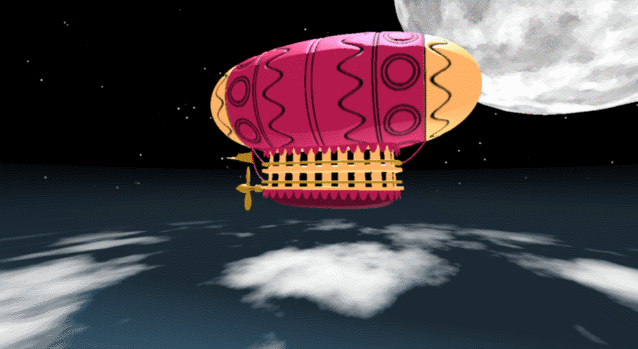
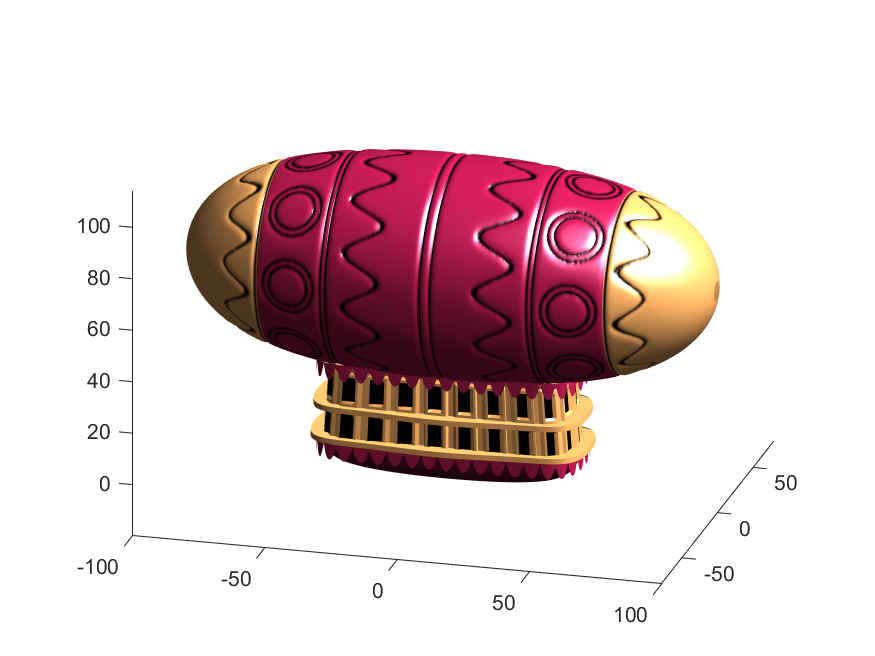
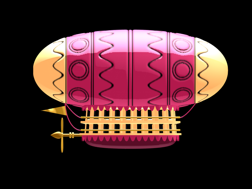
In the spirit of warming up for this year's minihack contest, I'm uploading a walkthrough for how to design an airship using pure Matlab script. This is commented and uncondensed; half of the challenge for the minihacks is how minimize characters. But, maybe it will give people some ideas.
The actual airship design is from one of my favorite original NES games that I played when I was a kid - Little Nemo: The Dream Master. The design comes from the intro of the game when Nemo sees the Slumberland airship leave for Slumberland:

(Snip from a frame of the opening scene in Capcom's game Little Nemo: The Dream Master, showing the Slumberland airship).
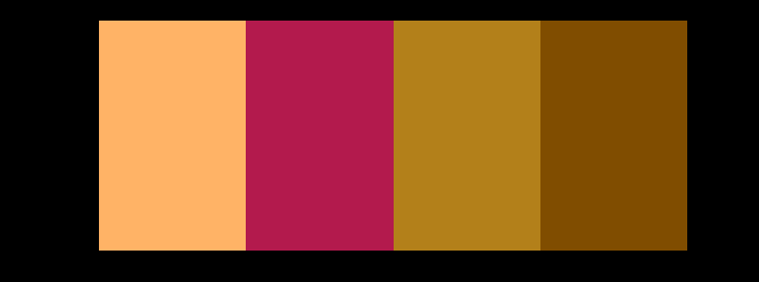
I spent hours playing this game with my two sisters, when we were little. It's fun and tough, but the graphics sparked the imagination. On to the code walkthrough, beginning with the color palette: these four colors are the only colors used for the airship:
c1=cat(3,1,.7,.4); % Cream color
c2=cat(3,.7,.1,.3); % Magenta
c3=cat(3,0.7,.5,.1); % Gold
c4=cat(3,.5,.3,0); % bronze
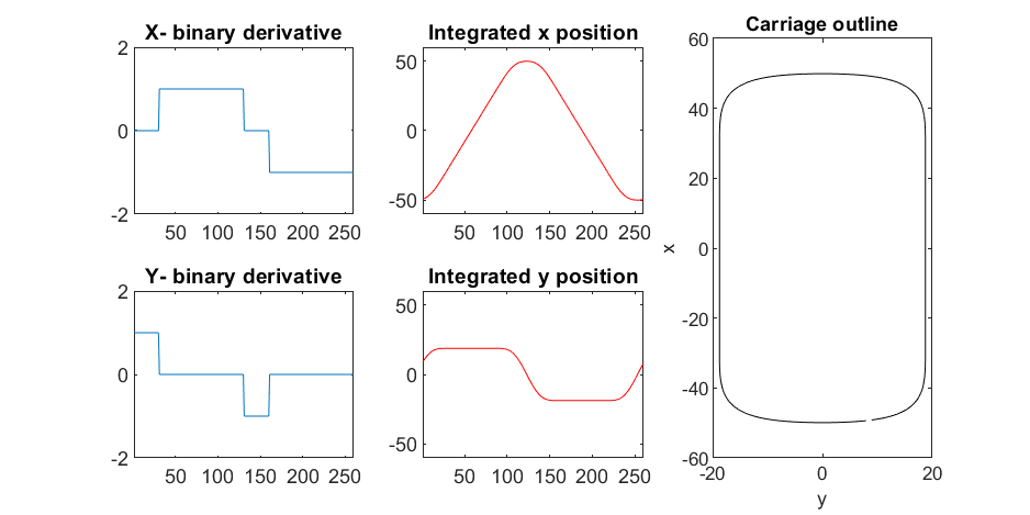
We start with the airship carriage body. We want something rectangular but smoothed on the corners. To do this we are going to start with the separate derivatives of the x and y components, which can be expressed using separate blocks of only three levels: [1, 0, -1]. You could integrate to create a rectangle, but if we smooth the derivatives prior to integrating we will get rounded edges. This is done in the following code:
% Binary components for x & y vectors
z=zeros(1,30);
o=ones(1,100);
% X and y vectors
x=[z,o,z,-o];
y=[1+z,1-o,z-1,1-o];
% Smoother function (fourier / circular)
s=@(x)ifft(fft(x).*conj(fft(hann(45)'/22,260)));
% Integrator function with replication and smoothing to form mesh matrices
u=@(x)repmat(cumsum(s(x)),[30,1]);
% Construct x and y components of carriage with offsets
x3=u(x)-49.35;
y3=u(y)+6.35;
y3 = y3*1.25; % Make it a little fatter
% Add a z-component to make the full set of matrices for creating a 3D
% surface:
z3=linspace(0,1,30)'.*ones(1,260)*30;
z3(14,:)=z3(15,:); % These two lines are for adding platforms
z3(2,:)=z3(3,:); % to the carriage, later.
Plotting x, y, and the top row of the smoothed, integrated, and replicated matrices x3 and y3 gives the following:
We now have the x and y components for a 3D mesh of the carriage, let's make it more interesting by adding a color scheme including doors, and texture for the trim around the doors. Let's also add platforms beneath the doors for passengers to walk on.
Starting with the color values, let's make doors by convolving points in a color-matrix by a door shaped function.
m=0*z3; % Image matrix that will be overlayed on carriage surface
m(7,10:12:end)=1; % Door locations (lower deck)
m(21,10:12:end)=1; % Door locations (upper deck)
drs = ones(9, 5); % Door shape
m=1-conv2(m,ones(9,5),'same'); % Applying
To add the trim, we will convolve matrix "m" (the color matrix) with a square function, and look for values that lie between the extrema. We will use this to create a displacement function that bumps out the -x, and -y values of the carriage surface in intermediary polar coordinate format.
rm=conv2(m,ones(5)/25,'same'); % Smoothing the door function
rm(~m)=0; % Preserving only the region around the doors
rds=0*m; % Radial displacement function
rds(rm<1&rm>0)=1; % Preserving region around doors
rds(m==0)=0;
rds(13:14,:)=6; % Adding walkways
rds(1:2,:)=6;
% Apply radial displacement function
[th,rd]=cart2pol(x3,y3);
[x3T,y3T]=pol2cart(th,(rd+rds)*.89);
If we plot the color function (m) and radial displacement function (rds) we get the following:
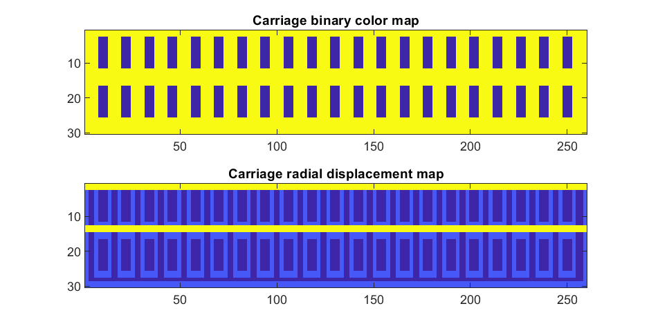
In the upper plot you can see the doors, and in the bottom map you can see the walk way and door trim.
Next, we are going to add some flags draped from the bottom and top of the carriage. We are going to recycle the values in "z3" to do this, by multiplying that matrix with the absolute value of a sine-wave, squished a bit with the soft-clip erf() function.
We add a keel to the airship carriage using a canonical sphere turned on its side, again using the soft-clip erf() function to make it roughly rectangular in x and y, and multiplying with a vector that is half nan's to make the top half transparent.
At this point, since we are beginning the plotting of the ship, we also need to create our hgtransform objects. These allow us to move all of the components of the airship in unison, and also link objects with pivot points to the airship, such as the propeller.
% Now we need some flags extending around the top and bottom of the
% carriage. We can do this my multiplying the height function (z3) with the
% absolute value of a sine-wave, rounded with a compression function
% (erf() in this case);
g=-z3.*erf(abs(sin(linspace(0,40*pi,260))))/4; % Flags
% Also going to add a slight taper to the carriage... gives it a nice look
tp=linspace(1.05,1,30)';
% Finally, plotting. Plot the carriage with the color-map for the doors in
% the cream color, than the flags in magenta. Attach them both to transform
% objects for movement.
% Set up transform objects. 2 moving parts:
% 1) The airship itself and all sub-components
% 2) The propellor, which attaches to the airship and spins on its axis.
hold on;
P=hgtransform('Parent',gca); % Ship
S=hgtransform('Parent',P); % Prop
surf(x3T.*tp,y3T,z3,c1.*m,'Parent',P);
surf(x3,y3,g,c2.*rd./rd, 'Parent', P);
surf(x3,y3,g+31,c2.*rd./rd, 'Parent', P);
axis equal
% Now add the keel of the airship. Will use a canonical sphere and the
% erf() compression function to square off.
[x,y,z]=sphere(99);
mk=round(linspace(-1,1).^2+.3); % This function makes the top half of the sphere nan's for transparency.
surf(50*erf(1.4*z),15*erf(1.4*y),13*x.*mk./mk-1,.5*c2.*z./z, 'Parent', P);
% The carriage is done. Now we can make the blimp above it.
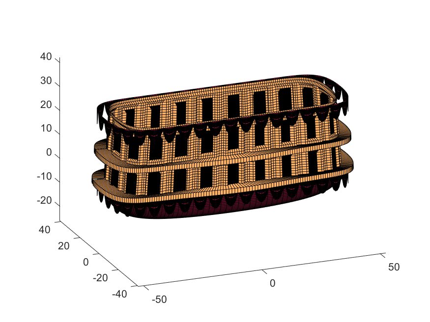
We haven't adjusted the shading of the image yet, but you can see the design features that have been created:
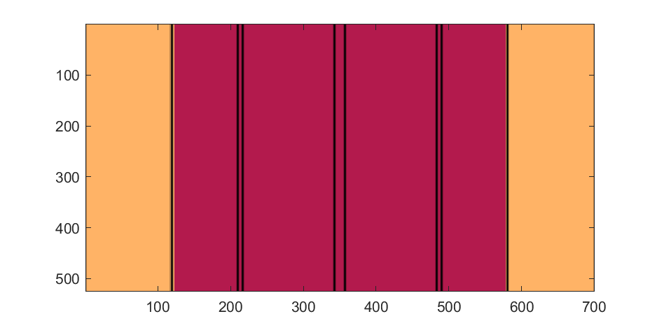
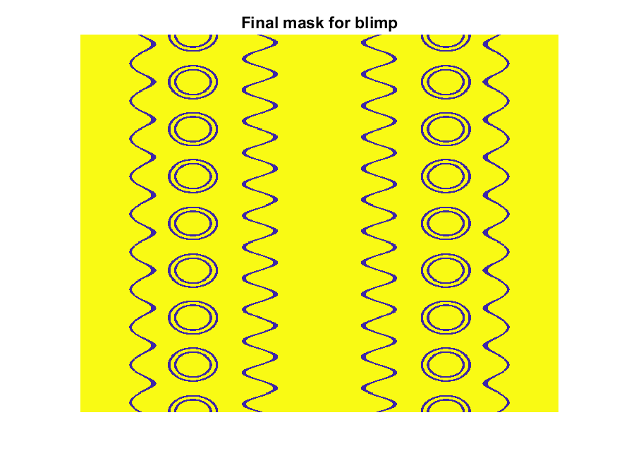
Next, we start working on the blimp. This is going to use a few more vertices & faces. We are going to use a tapered cylinder for this part, and will start by making the overlaid image, which will have 2 colors plus radial rings, circles, and squiggles for ornamentation.
M=525; % Blimp (matrix dimensions)
N=700;
% Assign the blimp the cream and magenta colors
t=122; % Transition point
b=ones(M,N,3); % Blimp color map template
bc=b.*c1; % Blimp color map
bc(:,t+1:end-t,:)=b(:,t+1:end-t,:).*c2;
% Add axial rings around blimp
l=[.17,.3,.31,.49];
l=round([l,1-fliplr(l)]*N); % Mirroring
lnw=ones(1,N); % Mask
lnw(l)=0;
lnw=rescale(conv(lnw,hann(7)','same'));
bc=bc.*lnw;
% Now add squiggles. We're going to do this by making an even function in
% the x-dimension (N, 725) added with a sinusoidal oscillation in the
% y-dimension (M, 500), then thresholding.
r=sin(linspace(0, 2*pi, M)*10)'+(linspace(-1, 1, N).^6-.18)*15;
q=abs(r)>.15;
r=sin(linspace(0, 2*pi, M)*12)'+(abs(linspace(-1, 1, N))-.25)*15;
q=q.*(abs(r)>.15);
% Now add the circles on the blimp. These will be spaced evenly in the
% polar angle dimension around the axis. We will have 9. To make the
% circles, we will create a cone function with a peak at the center of the
% circle, and use thresholding to create a ring of appropriate radius.
hs=[1,.75,.5,.25,0,-.25,-.5,-.75,-1]; % Axial spacing of rings
% Cone generation and ring loop
xy= @(h,s)meshgrid(linspace(-1, 1, N)+s*.53,(linspace(-1, 1, M)+h)*1.15);
w=@(x,y)sqrt(x.^2+y.^2);
for n=1:9
h=hs(n);
[xx,yy]=xy(h,-1);
r1=w(xx,yy);
[xx,yy]=xy(h,1);
r2=w(xx,yy);
b=@(x,y)abs(y-x)>.005;
q=q.*b(.1,r1).*b(.075,r1).*b(.1,r2).*b(.075,r2);
end
The figures below show the color scheme and mask used to apply the squiggles and circles generated in the code above:
Finally, for the colormap we are going to smooth the binary mask to avoid hard transitions, and use it to to add a "puffy" texture to the blimp shape. This will be done by diffusing the mask iteratively in a loop with a non-linear min() operator.
% 2D convolution function
ff=@(x)circshift(ifft2(fft2(x).*conj(fft2(hann(7)*hann(7)'/9,M,N))),[3,3]);
q=ff(q); % Smooth our mask function
hh=rgb2hsv(q.*bc); % Convert to hsv: we are going to use the value
% component for radial displacement offsets of the
% 3D blimp structure.
rd=hh(:,:,3); % Value component
for n=1:10
rd=min(rd,ff(rd)); % Diffusing the value component for a puffy look
end
rd=(rd+35)/36; % Make displacements effects small
% Now make 3D blimp manifold using "cylinder" canonical shape
[x,y,z]=cylinder(erf(sin(linspace(0,pi,N)).^.5)/4,M-1); % First argument is the blimp taper
[t,r]=cart2pol(x, y);
[x2,y2]=pol2cart(t, r.*rd'); % Applying radial displacment from mask
s=200;
% Plotting the blimp
surf(z'*s-s/2, y2'*s, x2'*s+s/3.9+15, q.*bc,'Parent',P);
Notice that the parent of the blimp surface plot is the same as the carriage (e.g. hgtransform object "P"). Plotting at this point using flat shading and adding some lighting gives the image below:
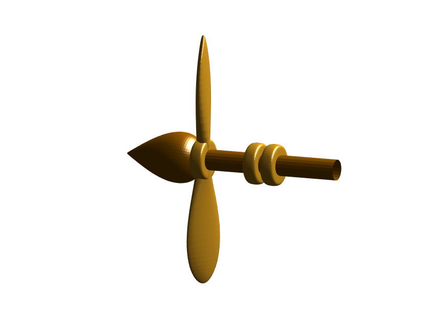
Next, we need to add a propeller so it can move. This will include the creation of a shaft using the cylinder() function. The rest of the pieces (the propeller blades, collars and shaft tip) all use the same canonical sphere with distortions applied using various math functions. Note that when the propeller is made it is linked to hgtransform object "S" rather than "P." This will allow the propeller to rotate, but still be joined to the airship.
% Next, the propeller. First, we start with the shaft. This is a simple
% cylinder. We add an offset variable and a scale variable to move our
% propeller components around, as well.
shx = -70; % This is our x-shifter for components
scl = 3; % Component size scaler
[x,y,z]=cylinder(1, 20); % Canonical cylinder for prop shaft.
p(1)=surf(-scl*(z-1)*7+shx,scl*x/2,scl*y/2,0*x+c4,'Parent',P); % Prop shaft
% Now the propeller. This is going to be made from a distorted sphere.
% The important thing here is that it is linked to the "S" hgtransform
% object, which will allow it to rotate.
[x,y,z]=sphere(50);
a=(-1:.04:1)';
x2=(x.*cos(a)-y/3.*sin(a)).*(abs(sin(a*2))*2+.1);
y2=(x.*sin(a)+y/3.*cos(a));
p(2)=surf(-scl*y2+shx,scl*x2,scl*z*6,0*x+c3,'Parent',S);
% Now for the prop-collars. You can see these on the shaft in the NES
% animation. These will just be made by using the canonical sphere and the
% erf() activation function to square it in the x-dimension.
g=erf(z*3)/3;
r=@(g)surf(-scl*g+shx,scl*x,scl*y,0*x+c3,'Parent',P);
r(g);
r(g-2.8);
r(g-3.7);
% Finally, the prop shaft tip. This will just be the sphere with a
% taper-function applied radially.
t=1.7*cos(0:.026:1.3)'.^2;
p(3)=surf(-(z*2+2)*scl + shx,x.*t*scl,y.*t*scl, 0*x+c4,'Parent',P);
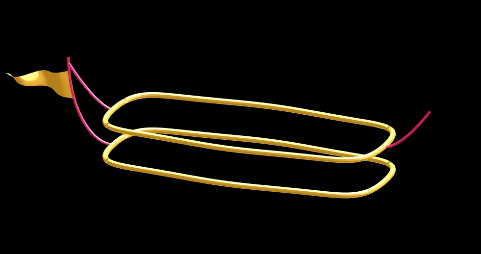
Now for some final details including the ropes to the blimp, a flag hung on one of the ropes, and railings around the walkways so that passengers don't plummet to their doom. This will make use of the ad-hoc "ropeG" function, which takes a 3D vector of points and makes a conforming cylinder around it, so that you get lighting functions etc. that don't work on simple lines. This function is added to the script at the end to do this:
% Rope function for making a 3D curve have thickness, like a rope.
% Inputs:
% - xyz (3D curve vector, M points in 3 x M format)
% - N (Number of radial points in cylinder function around the curve
% - W (Width of the rope)
%
% Outputs:
% - xf, yf, zf (Matrices that can be used with surf())
function [xf, yf, zf] = RopeG(xyz, N, W)
% Canonical cylinder with N points in circumference
[xt,yt,zt] = cylinder(1, N);
% Extract just the first ring and make (W) wide
xyzt = [xt(1, :); yt(1, :); zt(1, :)]*W;
% Get local orientation vector between adjacent points in rope
dxyz = xyz(:, 2:end) - xyz(:, 1:end-1);
dxyz(:, end+1) = dxyz(:, end);
vcs = dxyz./vecnorm(dxyz);
% We need to orient circle so that its plane normal is parallel to
% xyzt. This is a kludgey way to do that.
vcs2 = [ones(2, size(vcs, 2)); -(vcs(1, :) + vcs(2, :))./(vcs(3, :)+0.01)];
vcs2 = vcs2./vecnorm(vcs2);
vcs3 = cross(vcs, vcs2);
p = @(x)permute(x, [1, 3, 2]);
rmats = [p(vcs3), p(vcs2), p(vcs)];
% Create surface
xyzF = pagemtimes(rmats, xyzt) + permute(xyz, [1, 3, 2]);
% Outputs for surf format
xf = squeeze(xyzF(1, :, :));
yf = squeeze(xyzF(2, :, :));
zf = squeeze(xyzF(3, :, :));
end
Using this function we can define the ropes and balconies. Note that the balconies simply recycle one of the rows of the original carriage surface, defining the outer rim of the walkway, but bumping up in the z-dimension.
cb=-sqrt(1-linspace(1, 0, 100).^2)';
c1v=[linspace(-67, -51)', 0*ones(100,1),cb*30+35];
c2v=[c1v(:,1),c1v(:,2),(linspace(1,0).^1.5-1)'*15+33];
c3v=c2v.*[-1,1,1];
[xr,yr,zr]=RopeG(c1v', 10, .5);
surf(xr,yr,zr,0*xr+c2,'Parent',P);
[xr,yr,zr]=RopeG(c2v', 10, .5);
surf(xr,yr,zr,0*zr+c2,'Parent',P);
[xr,yr,zr]=RopeG(c3v', 10, .5);
surf(xr,yr,zr,0*zr+c2,'Parent',P);
% Finally, balconies would add a nice touch to the carriage keep people
% from falling to their death at 10,000 feet.
[rx,ry,rz]=RopeG([x3T(14, :); y3T(14,:); 0*x3T(14,:)+18]*1.01, 10, 1);
surf(rx,ry,rz,0*rz+cat(3,0.7,.5,.1),'Parent',P);
surf(rx,ry,rz-13,0*rz+cat(3,0.7,.5,.1),'Parent',P);
And, very last, we are going to add a flag attached to the outer cable. Let's make it flap in the wind. To make it we will recycle the z3 matrix again, but taper it based on its x-value. Then we will sinusoidally oscillate the flag in the y dimension as a function of x, constraining the y-position to be zero where it meets the cable. Lastly, we will displace it quadratically in the x-dimension as a function of z so that it lines up nicely with the rope. The phase of the sine-function is modified in the animation loop to give it a flapping motion.
h=linspace(0,1);
sc=10;
[fx,fz]=meshgrid(h,h-.5);
F=surf(sc*2.5*fx-90-2*(fz+.5).^2,sc*.3*erf(3*(1-h)).*sin(10*fx+n/5),sc*fz.*h+25,0*fx+c3,'Parent',P);
Plotting just the cables and flag shows:
Putting all the pieces together reveals the full airship:
A note about lighting: lighting and material properties really change the feel of the image you create. The above picture is rendered in a cartoony style by setting the specular exponent to a very low value (1), and adding lots of diffuse and ambient reflectivity as well. A light below the airship was also added, albeit with lower strength. Settings used for this plot were:
shading flat
view([0, 0]);
L=light;
L.Color = [1,1,1]/4;
light('position', [0, 0.5, 1], 'color', [1,1,1]);
light('position', [0, 1, -1], 'color', [1, 1, 1]/5);
material([1, 1, .7, 1])
set(gcf, 'color', 'k');
axis equal off
What about all the rest of the stuff (clouds, moon, atmospheric haze etc.) These were all (mostly) recycled bits from previous minihack entries. The clouds were made using power-law noise as explained in Adam Danz' blog post. The moon was borrowed from moonrun, but with an increased number of points. Atmospheric haze was recycled from Matlon5. The rest is just camera angles, hgtransform matrix updates, and updating alpha-maps or vertex coordinates.
Finally, the use of hann() adds the signal processing toolbox as a dependency. To avoid this use the following anonymous function:
hann = @(x)-cospi(linspace(0,2,x)')/2+.5;
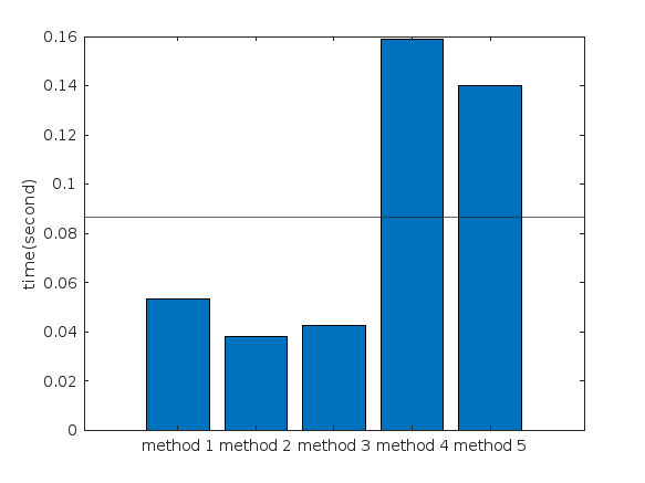
Create a struct arrays where each struct has field names "a," "b," and "c," which store different types of data. What efficient methods do you have to assign values from individual variables "a," "b," and "c" to each struct element? Here are five methods I've provided, listed in order of decreasing efficiency. What do you think?
Create an array of 10,000 structures, each containing each of the elements corresponding to the a,b,c variables.
num = 10000;
a = (1:num)';
b = string(a);
c = rand(3,3,num);
Here are the methods;
%% method1
t1 =tic;
s = struct("a",[], ...
"b",[], ...
"c",[]);
s1 = repmat(s,num,1);
for i = 1:num
s1(i).a = a(i);
s1(i).b = b(i);
s1(i).c = c(:,:,i);
end
t1 = toc(t1);
%% method2
t2 =tic;
for i = num:-1:1
s2(i).a = a(i);
s2(i).b = b(i);
s2(i).c = c(:,:,i);
end
t2 = toc(t2);
%% method3
t3 =tic;
for i = 1:num
s3(i).a = a(i);
s3(i).b = b(i);
s3(i).c = c(:,:,i);
end
t3 = toc(t3);
%% method4
t4 =tic;
ct = permute(c,[3,2,1]);
t = table(a,b,ct);
s4 = table2struct(t);
t4 = toc(t4);
%% method5
t5 =tic;
s5 = struct("a",num2cell(a),...
"b",num2cell(b),...
"c",squeeze(mat2cell(c,3,3,ones(num,1))));
t5 = toc(t5);
%% plot
bar([t1,t2,t3,t4,t5])
xtickformat('method %g')
ylabel("time(second)")
yline(mean([t1,t2,t3,t4,t5]))
As far as I know, starting from MATLAB R2024b, the documentation is defaulted to be accessed online. However, the problem is that every time I open the official online documentation through my browser, it defaults or forcibly redirects to the documentation hosted site for my current geographic location, often with multiple pop-up reminders, which is very annoying!

Suggestion: Could there be an option to set preferences linked to my personal account so that the documentation defaults to my chosen language preference without having to deal with “forced reminders” or “forced redirection” based on my geographic location? I prefer reading the English documentation, but the website automatically redirects me to the Chinese documentation due to my geolocation, which is quite frustrating!
----------------2024.12.13 update-----------------
Although the above issue was resolved by technical support, subsequent redirects are still causing severe delays...
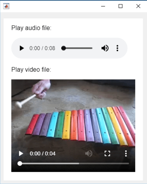
In the past two years, MATHWORKS has updated the image viewer and audio viewer, giving them a more modern interface with features like play, pause, fast forward, and some interactive tools that are more commonly found in typical third-party players. However, the video player has not seen any updates. For instance, the Video Viewer or vision.VideoPlayer could benefit from a more modern player interface. Perhaps I haven't found a suitable built-in player yet. It would be great if there were support for custom image processing and audio processing algorithms that could be played in a more modern interface in real time.
Additionally, I found it quite challenging to develop a modern video player from scratch in App Designer.(If there's a video component for that that would be great)
-----------------------------------------------------------------------------------------------------------------
BTW,the following picture shows the built-in function uihtml function showing a more modern playback interface with controls for play, pause and so on. But can not add real-time image processing algorithms within it.
I was browsing the MathWorks website and decided to check the Cody leaderboard. To my surprise, William has now solved 5,000 problems. At the moment, there are 5,227 problems on Cody, so William has solved over 95%. The next competitor is over 500 problems behind. His score is also clearly the highest, approaching 60,000.
D.R. Kaprekar was a self taught recreational mathematician, perhaps known mostly for some numbers that bear his name.
Today, I'll focus on Kaprekar's constant (as opposed to Kaprekar numbers.)
The idea is a simple one, embodied in these 5 steps.
1. Take any 4 digit integer, reduce to its decimal digits.
2. Sort the digits in decreasing order.
3. Flip the sequence of those digits, then recompose the two sets of sorted digits into 4 digit numbers. If there were any 0 digits, they will become leading zeros on the smaller number. In this case, a leading zero is acceptable to consider a number as a 4 digit integer.
4. Subtract the two numbers, smaller from the larger. The result will always have no more than 4 decimal digits. If it is less than 1000, then presume there are leading zero digits.
5. If necessary, repeat the above operation, until the result converges to a stable result, or until you see a cycle.
Since this process is deterministic, and must always result in a new 4 digit integer, it must either terminate at either an absorbing state, or in a cycle.
For example, consider the number 6174.
7641 - 1467
We get 6174 directly back. That seems rather surprising to me. But even more interesting is you will find all 4 digit numbers (excluding the pure rep-digit nmbers) will always terminate at 6174, after at most a few steps. For example, if we start with 1234
4321 - 1234
8730 - 0378
8532 - 2358
and we see that after 3 iterations of this process, we end at 6174. Similarly, if we start with 9998, it too maps to 6174 after 5 iterations.
9998 ==> 999 ==> 8991 ==> 8082 ==> 8532 ==> 6174
Why should that happen? That is, why should 6174 always drop out in the end? Clearly, since this is a deterministic proces which always produces another 4 digit integer (Assuming we treat integers with a leading zero as 4 digit integers), we must either end in some cycle, or we must end at some absorbing state. But for all (non-pure rep-digit) starting points to end at the same place, it seems just a bit surprising.
I always like to start a problem by working on a simpler problem, and see if it gives me some intuition about the process. I'll do the same thing here, but with a pair of two digit numbers. There are 100 possible two digit numbers, since we must treat all one digit numbers as having a "tens" digit of 0.
N = (0:99)';
Next, form the Kaprekar mapping for 2 digit numbers. This is easier than you may think, since we can do it in a very few lines of code on all possible inputs.
Ndig = dec2base(N,10,2) - '0';
Nmap = sort(Ndig,2,'descend')*[10;1] - sort(Ndig,2,'ascend')*[10;1];
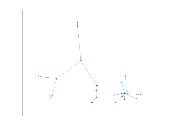
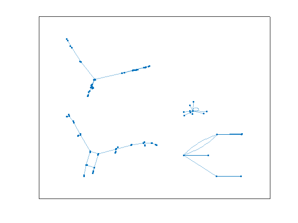
I'll turn it into a graph, so we can visualize what happens. It also gives me an excuse to employ a very pretty set of tools in MATLAB.
G2 = graph(N+1,Nmap+1,[],cellstr(dec2base(N,10,2)));
plot(G2)
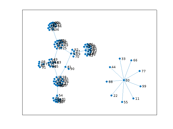
Do you see what happens? All of the rep-digit numbers, like 11, 44, 55, etc., all map directly to 0, and they stay there, since 0 also maps into 0. We can see that in the star on the lower right.
G2cycles = cyclebasis(G2)
G2cycles{1}
All other numbers eventually end up in the cycle:
G2cycles{2}
That is
81 ==> 63 ==> 27 ==> 45 ==> 09 ==> and back to 81
looping forever.
Another way of trying to visualize what happens with 2 digit numbers is to use symbolics. Thus, if we assume any 2 digit number can be written as 10*T+U, where I'll assume T>=U, since we always sort the digits first
syms T U
(10*T + U) - (10*U+T)
So after one iteration for 2 digit numbers, the result maps ALWAYS to a new 2 digit number that is divisible by 9. And there are only 10 such 2 digit numbers that are divisible by 9. So the 2-digit case must resolve itself rather quickly.
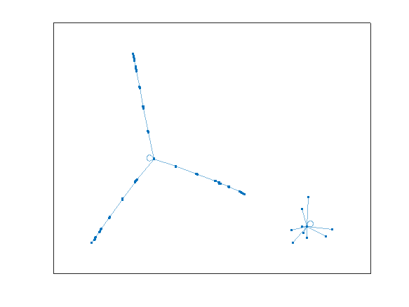
What happens when we move to 3 digit numbers? Note that for any 3 digit number abc (without loss of generality, assume a >= b >= c) it almost looks like it reduces to the 2 digit probem, aince we have abc - cba. The middle digit will always cancel itself in the subtraction operation. Does that mean we should expect a cycle at the end, as happens with 2 digit numbers? A simple modification to our previous code will tell us the answer.
N = (0:999)';
Ndig = dec2base(N,10,3) - '0';
Nmap = sort(Ndig,2,'descend')*[100;10;1] - sort(Ndig,2,'ascend')*[100;10;1];
G3 = graph(N+1,Nmap+1,[],cellstr(dec2base(N,10,2)));
plot(G3)
This one is more difficult to visualize, since there are 1000 nodes in the graph. However, we can clearly see two disjoint groups.
We can use cyclebasis to tell us the complete story again.
G3cycles = cyclebasis(G3)
G3cycles{:}
And we see that all 3 digit numbers must either terminate at 000, or 495. For example, if we start with 181, we would see:
811 - 118
963 - 369
954 - 459
It will terminate there, forever trapped at 495. And cyclebasis tells us there are no other cycles besides the boring one at 000.
What is the maximum length of any such path to get to 495?
D3 = distances(G3,496) % Remember, MATLAB uses an index origin of 1
D3(isinf(D3)) = -inf; % some nodes can never reach 495, so they have an infinite distance
plot(D3)
The maximum number of steps to get to 495 is 6 steps.
find(D3 == 6) - 1
So the 3 digit number 100 required 6 iterations to eventually reach 495.
shortestpath(G3,101,496) - 1
I think I've rather exhausted the 3 digit case. It is time now to move to the 4 digit problem, but we've already done all the hard work. The same scheme will apply to compute a graph. And the graph theory tools do all the hard work for us.
N = (0:9999)';
Ndig = dec2base(N,10,4) - '0';
Nmap = sort(Ndig,2,'descend')*[1000;100;10;1] - sort(Ndig,2,'ascend')*[1000;100;10;1];
G4 = graph(N+1,Nmap+1,[],cellstr(dec2base(N,10,2)));
plot(G4)
cyclebasis(G4)
ans{:}
And here we see the behavior, with one stable final point, 6174 as the only non-zero ending state. There are no circular cycles as we had for the 2-digit case.
How many iterations were necessary at most before termination?
D4 = distances(G4,6175);
D4(isinf(D4)) = -inf;
plot(D4)
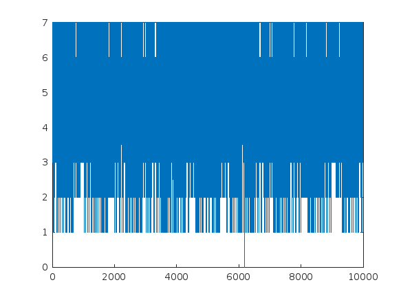
The plot tells the story here. The maximum number of iterations before termination is 7 for the 4 digit case.
find(D4 == 7,1,'last') - 1
shortestpath(G4,9986,6175) - 1
Can you go further? Are there 5 or 6 digit Kaprekar constants? Sadly, I have read that for more than 4 digits, things break down a bit, there is no 5 digit (or higher) Kaprekar constant.
We can verify that fact, at least for 5 digit numbers.
N = (0:99999)';
Ndig = dec2base(N,10,5) - '0';
Nmap = sort(Ndig,2,'descend')*[10000;1000;100;10;1] - sort(Ndig,2,'ascend')*[10000;1000;100;10;1];
G5 = graph(N+1,Nmap+1,[],cellstr(dec2base(N,10,2)));
plot(G5)
cyclebasis(G5)
ans{:}
The result here are 4 disjoint cycles. Of course the rep-digit cycle must always be on its own, but the other three cycles are also fully disjoint, and are of respective length 2, 4, and 4.
I've been working on some matrix problems recently(Problem 55225)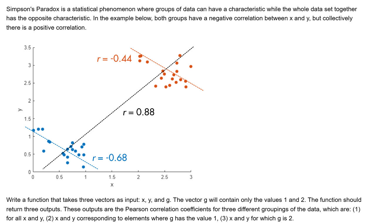
and this is my code
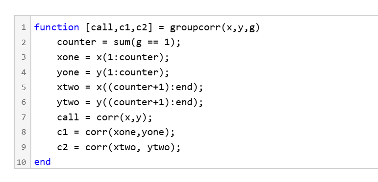
It turns out that "Undefined function 'corr' for input arguments of type 'double'." However, should't the input argument of "corr" be column vectors with single/double values? What's even going on there?
isequaln exists to return true when NaN==NaN.
unique treats NaN==NaN as false (as it should) requiring NaN to be replaced if NaN is not considered unique in a particular application. In my application, I am checking uniqueness of table rows using [table_unique,index_unique]=unique(table,"rows","sorted") and would prefer to keep NaN as NaN or missing in table_unique without the overhead of replacing it with a dummy value then replacing it again. Dummy values also have the risk of matching existing values in the table, requiring first finding a dummy value that is not in the table.
uniquen (similar to isequaln) would be more eloquent.
Please point out if I am missing something!
您也可以从以下列表中选择网站:
美洲
- América Latina (Español)
- Canada (English)
- United States (English)
欧洲
- Belgium (English)
- Denmark (English)
- Deutschland (Deutsch)
- España (Español)
- Finland (English)
- France (Français)
- Ireland (English)
- Italia (Italiano)
- Luxembourg (English)
- Netherlands (English)
- Norway (English)
- Österreich (Deutsch)
- Portugal (English)
- Sweden (English)
- Switzerland
- United Kingdom(English)
亚太
- Australia (English)
- India (English)
- New Zealand (English)
- 中国
- 日本Japanese (日本語)
- 한국Korean (한국어)