搜索
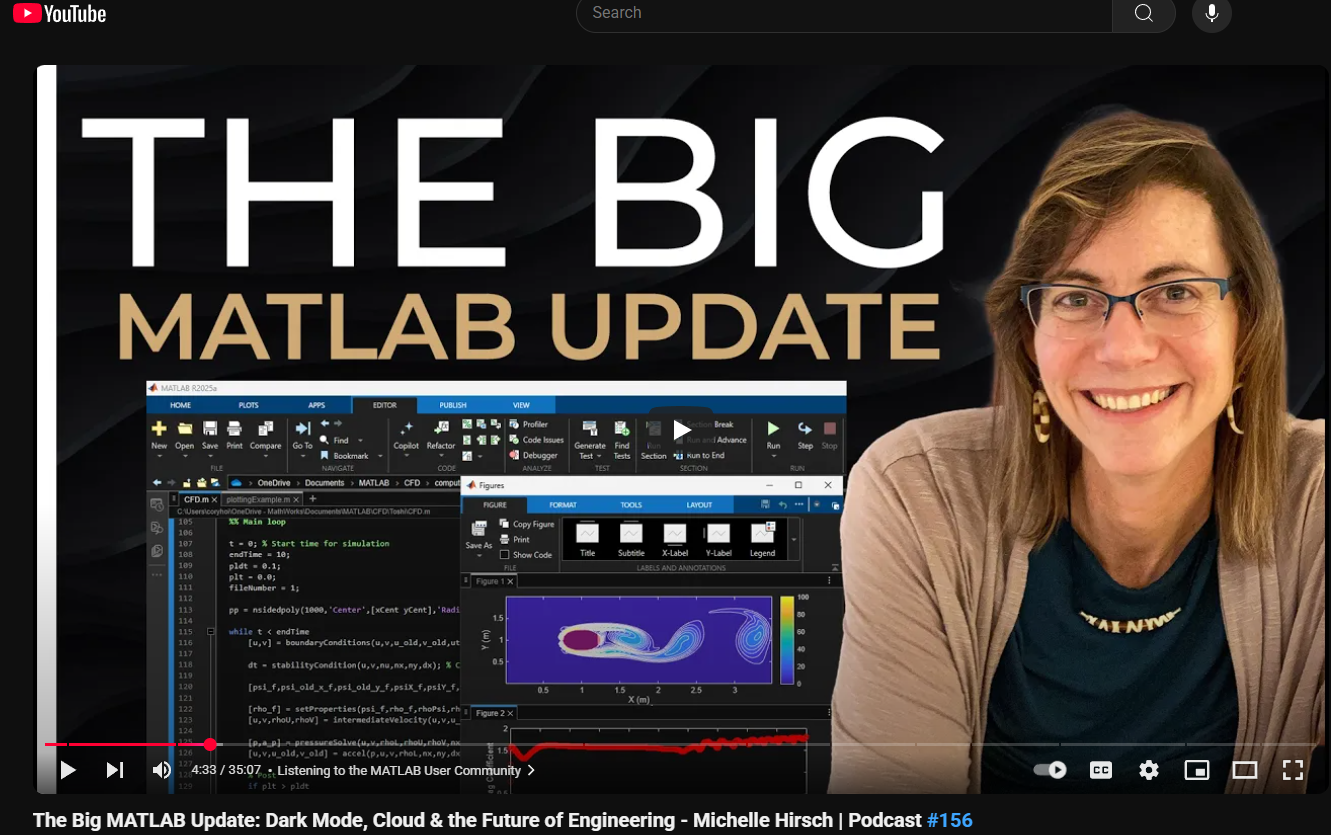
This just came out. @Michelle Hirsch spoke to Jousef Murad and answer his questions about the big change in the desktop in R2025a and explained what was going on behind the scene. Enjoy!
The Big MATLAB Update: Dark Mode, Cloud & the Future of Engineering - Michelle Hirsch
These got released last week and the process for using them on your local machine with MATLAB is very similar to how you use the local deepseek models as I demonstrated in my February blog post How to run local DeepSeek models and use them with MATLAB » The MATLAB Blog - MATLAB & Simulink
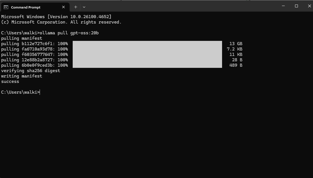
You need Ollama and the LLMs with MATLAB package installed (Details on how to do this in the blog post above). Then you run the following in your operating systems' command line
ollama pull gpt-oss:20b
Over to MATLAB and set up a chat session
>> chat = ollamaChat("gpt-oss:20b")
chat =
ollamaChat with properties:
ModelName: "gpt-oss:20b"
Endpoint: "127.0.0.1:11434"
TopK: Inf
MinP: 0
TailFreeSamplingZ: 1
Temperature: 1
TopP: 1
StopSequences: [0×0 string]
TimeOut: 120
SystemPrompt: []
ResponseFormat: "text"
FunctionNames: []
txt = generate(chat,"Who are you?")
txt =
"I’m ChatGPT – a conversational AI developed by OpenAI. My core is the GPT‑4 language model, which has been trained on a massive mix of text from books, websites, articles and other sources to understand and generate human‑like language. I don’t have feelings, consciousness, or a personal identity; I’m a tool that can help answer questions, brainstorm ideas, explain concepts, draft text, and more. My goal is to understand the context you give me and respond in a helpful, accurate and safe way. If there’s something specific you’d like to know or do, just let me know!"
This is the smaller of the two, new open models and it is bringing my aging desktop to its knees. My GPU is too small to do the work so I think everything is happening on the CPU and its slooooow. Will try on my Mac next
Let me know if you try this out!
Long before I joined MathWorks, I was a member of the academic Research Software Engineering (RSE) community where part of my mission was to introduce basic software engineering concepts to the research community. Things like version control, testing and even simply writing code instead of using only pointy-clicky GUIs before copying and pasting the results plot into a word document. I've seen things..........*shudders*
The RSE movement is still going very strong and I am elated that MathWorks is increasingly interacting with it. One example of such interaction is a video tutorial contributed by my colleauge @Mihaela Jarema to a comminity seminar series called 'A summer of Testing' It's linked to below
The video assumes you've never run a test before and gently guides you through the principles. Along the way you'll learn about some of MATLAB's superb testing capabilities. Things like
- Unit testing Framework
- Test Browser App
- Code Coverage
- Test Fixtures (Setup and teardown)
- Test driven devellopment
- Function argument validation
- CI/CD using GitHub actions
Go check out out.

Hey cody fellows :-) !
I recently created two problem groups, but as you can see I struggle to set their cover images :
What is weird given :
- I already did it successfully twice in the past for my previous groups ;
- If you take one problem specifically, Problem 60984. Mesh the icosahedron for instance, you can normally see the icon of the cover image in the top right hand corner, can't you ?
- I always manage to set cover images to my contributions (mostly in the filexchange).
I already tried several image formats, included .png 4/3 ratio, but still the cover images don't set.
Could you please help me to correctly set my cover images ?
Thank you.
Nicolas
I just wanted here to share a link to some .gif animations I created over the years with Matlab :-)
I think gif animations are great supports for scientific diffusion.
Hello to all!
I would like to share with the Matlab and Simulink community this video about Neural Networks in Simulink.
This is a series of videos that use a multilayer perceptron implemented in Simulink as a case study. Why Simulink? Because it's a visual and intuitive modeling tool, you can see the forward propagation of this network and better understand the flow. The objective of this series is to show the implementation using Simulink for both simulation and Arduino, as well as its training using Matlab and Matlab with Deep Learning Toolbox, and a video of training with Python.
The video is in Spanish, but the Simulink model is available in English for the entire community; subtitles are also available.
The files are located in the first comment of each video. We hope you find it interesting and enjoyable. Best regards!
Here I share the link to the first video.
In many parts of Africa, particularly in technical universities and engineering institutes, physical laboratories are scarce or poorly equipped. This reality deeply limits the hands-on experience students deserve, especially in fields like control systems, signal processing, power electronics, and fluid mechanics.
But MATLAB and Simulink can fill part of this gap.
As an educator and researcher, I’ve made it my mission to promote MATLAB as a didactic simulation environment that brings real-world experimentation into the virtual space—affordable, accessible, and scalable. Whether simulating dynamic systems, visualizing electromagnetic fields, or tuning PID controllers interactively, students can develop strong intuition without needing costly hardware.
🔧 I’ve used MATLAB to teach:
- Power systems and control theory without needing real generators or oscilloscopes,
- Hydrology and environmental modeling without field sensors,
- Robotics and AI concepts even where no robot is available.
🌍 This is more than a tool for me. It’s a bridge between educational ambition and limited infrastructure.
I dream of creating MATLAB-based virtual laboratories across African institutions. And I know I’m not alone.
Is anyone else here working on similar goals in under-resourced regions? Let’s connect and make it real.
— Patrick K.N.
As someone who grew up programming in C#, I often find myself wishing for a tighter, more native integration between MATLAB and C#.
There’s so much I dream of doing—leveraging the power of Simulink models or MATLAB’s advanced numerical libraries inside my .NET desktop or web applications. Of course, I know there are some workarounds: COM automation, MATLAB Engine API for .NET, or using MATLAB Compiler SDK… but let’s be honest: it’s not quite as seamless as I’d hope.
I imagine a world where:
- I could directly call MATLAB functions from C# as if they were .NET assemblies, without middleware.
- Simulink blocks could generate portable C# code (not just C/C++).
- MATLAB UI components could be embedded in WPF/WinForms apps natively.
Until then... we make do with what we have. But the vision remains.
Anyone else here trying to bridge MATLAB and C# in their workflow? I’d love to hear your experiences or ideas!
— Patrick K.N.
I found some beautiful computational art made by a developer called @yuruyurau who used a language called Processing. Unfortunately, I know very little about this language so I asked Claude to convert it to MATLAB for me.
Give it a try yourself and show me what you come up with.
Details here: Pair programming with Claude to produce computational art in MATLAB » The MATLAB Blog - MATLAB & Simulink

I have started a blog series on the history of image display in MATLAB. If this topic interests you, and if there is something in particular you would like me to address in the series, let me know.
t = turtle(); % Start a turtle
t.forward(100); % Move forward by 100
t.backward(100); % Move backward by 100
t.left(90); % Turn left by 90 degrees
t.right(90); % Tur right by 90 degrees
t.goto(100, 100); % Move to (100, 100)
t.turnto(90); % Turn to 90 degrees, i.e. north
t.speed(1000); % Set turtle speed as 1000 (default: 500)
t.pen_up(); % Pen up. Turtle leaves no trace.
t.pen_down(); % Pen down. Turtle leaves a trace again.
t.color('b'); % Change line color to 'b'
t.begin_fill(FaceColor, EdgeColor, FaceAlpha); % Start filling
t.end_fill(); % End filling
t.change_icon('person.png'); % Change the icon to 'person.png'
t.clear(); % Clear the Axes
classdef turtle < handle
properties (GetAccess = public, SetAccess = private)
x = 0
y = 0
q = 0
end
properties (SetAccess = public)
speed (1, 1) double = 500
end
properties (GetAccess = private)
speed_reg = 100
n_steps = 20
ax
l
ht
im
is_pen_up = false
is_filling = false
fill_color
fill_alpha
end
methods
function obj = turtle()
figure(Name='MATurtle', NumberTitle='off')
obj.ax = axes(box="on");
hold on,
obj.ht = hgtransform();
icon = flipud(imread('turtle.png'));
obj.im = imagesc(obj.ht, icon, ...
XData=[-30, 30], YData=[-30, 30], ...
AlphaData=(255 - double(rgb2gray(icon)))/255);
obj.l = plot(obj.x, obj.y, 'k');
obj.ax.XLim = [-500, 500];
obj.ax.YLim = [-500, 500];
obj.ax.DataAspectRatio = [1, 1, 1];
obj.ax.Toolbar.Visible = 'off';
disableDefaultInteractivity(obj.ax);
end
function home(obj)
obj.x = 0;
obj.y = 0;
obj.ht.Matrix = eye(4);
end
function forward(obj, dist)
obj.step(dist);
end
function backward(obj, dist)
obj.step(-dist)
end
function step(obj, delta)
if numel(delta) == 1
delta = delta*[cosd(obj.q), sind(obj.q)];
end
if obj.is_filling
obj.fill(delta);
else
obj.move(delta);
end
end
function goto(obj, x, y)
dx = x - obj.x;
dy = y - obj.y;
obj.turnto(rad2deg(atan2(dy, dx)));
obj.step([dx, dy]);
end
function left(obj, q)
obj.turn(q);
end
function right(obj, q)
obj.turn(-q);
end
function turnto(obj, q)
obj.turn(obj.wrap_angle(q - obj.q, -180));
end
function pen_up(obj)
if obj.is_filling
warning('not available while filling')
return
end
obj.is_pen_up = true;
end
function pen_down(obj, go)
if obj.is_pen_up
if nargin == 1
obj.l(end+1) = plot(obj.x, obj.y, Color=obj.l(end).Color);
else
obj.l(end+1) = go;
end
uistack(obj.ht, 'top')
end
obj.is_pen_up = false;
end
function color(obj, line_color)
if obj.is_filling
warning('not available while filling')
return
end
obj.pen_up();
obj.pen_down(plot(obj.x, obj.y, Color=line_color));
end
function begin_fill(obj, FaceColor, EdgeColor, FaceAlpha)
arguments
obj
FaceColor = [.6, .9, .6];
EdgeColor = [0 0.4470 0.7410];
FaceAlpha = 1;
end
if obj.is_filling
warning('already filling')
return
end
obj.fill_color = FaceColor;
obj.fill_alpha = FaceAlpha;
obj.pen_up();
obj.pen_down(patch(obj.x, obj.y, [1, 1, 1], ...
EdgeColor=EdgeColor, FaceAlpha=0));
obj.is_filling = true;
end
function end_fill(obj)
if ~obj.is_filling
warning('not filling now')
return
end
obj.l(end).FaceColor = obj.fill_color;
obj.l(end).FaceAlpha = obj.fill_alpha;
obj.is_filling = false;
end
function change_icon(obj, filename)
icon = flipud(imread(filename));
obj.im.CData = icon;
obj.im.AlphaData = (255 - double(rgb2gray(icon)))/255;
end
function clear(obj)
obj.x = 0;
obj.y = 0;
delete(obj.ax.Children(2:end));
obj.l = plot(0, 0, 'k');
obj.ht.Matrix = eye(4);
end
end
methods (Access = private)
function animated_step(obj, delta, q, initFcn, updateFcn)
arguments
obj
delta
q
initFcn = @() []
updateFcn = @(~, ~) []
end
dx = delta(1)/obj.n_steps;
dy = delta(2)/obj.n_steps;
dq = q/obj.n_steps;
pause_duration = norm(delta)/obj.speed/obj.speed_reg;
initFcn();
for i = 1:obj.n_steps
updateFcn(dx, dy);
obj.ht.Matrix = makehgtform(...
translate=[obj.x + dx*i, obj.y + dy*i, 0], ...
zrotate=deg2rad(obj.q + dq*i));
pause(pause_duration)
drawnow limitrate
end
obj.x = obj.x + delta(1);
obj.y = obj.y + delta(2);
end
function obj = turn(obj, q)
obj.animated_step([0, 0], q);
obj.q = obj.wrap_angle(obj.q + q, 0);
end
function move(obj, delta)
initFcn = @() [];
updateFcn = @(dx, dy) [];
if ~obj.is_pen_up
initFcn = @() initializeLine();
updateFcn = @(dx, dy) obj.update_end_point(obj.l(end), dx, dy);
end
function initializeLine()
obj.l(end).XData(end+1) = obj.l(end).XData(end);
obj.l(end).YData(end+1) = obj.l(end).YData(end);
end
obj.animated_step(delta, 0, initFcn, updateFcn);
end
function obj = fill(obj, delta)
initFcn = @() initializePatch();
updateFcn = @(dx, dy) obj.update_end_point(obj.l(end), dx, dy);
function initializePatch()
obj.l(end).Vertices(end+1, :) = obj.l(end).Vertices(end, :);
obj.l(end).Faces = 1:size(obj.l(end).Vertices, 1);
end
obj.animated_step(delta, 0, initFcn, updateFcn);
end
end
methods (Static, Access = private)
function update_end_point(l, dx, dy)
l.XData(end) = l.XData(end) + dx;
l.YData(end) = l.YData(end) + dy;
end
function q = wrap_angle(q, min_angle)
q = mod(q - min_angle, 360) + min_angle;
end
end
end
I would like to zoom directly on the selected region when using  on my image created with image or imagesc. First of all, I would recommend using image or imagesc and not imshow for this case, see comparison here: Differences between imshow() and image()? However when zooming Stretch-to-Fill behavior happens and I don't want that. Try range zoom to image generated by this code:
fig = uifigure;
ax = uiaxes(fig);
im = imread("peppers.png");
h = imagesc(im,"Parent",ax);
axis(ax,'tight', 'off')
I can fix that with manualy setting data aspect ratio:
daspect(ax,[1 1 1])
However, I need this code to run automatically after zooming. So I create zoom object and ActionPostCallback which is called everytime after I zoom, see zoom - ActionPostCallback.
z = zoom(ax);
z.ActionPostCallback = @(fig,ax) daspect(ax.Axes,[1 1 1]);
If you need, you can also create ActionPreCallback which is called everytime before I zoom, see zoom - ActionPreCallback.
z.ActionPreCallback = @(fig,ax) daspect(ax.Axes,'auto');
Code written and run in R2025a.
This week's Graphics and App Building blog article guides chart authors and app builders through the process of designing for a specific theme or creating theme-responsive charts and apps.
- Learn how dark theme may impacts charts and apps
- Discover best practices for theme-adaptive workflows
- Step-by-step examples for both script-based plots and advanced custom charts and UI components
- Discover new tools like ThemeChangedFcn, getTheme, and fliplightness
I'm planning to start a personal scientific software project. I used to be familiar with Matlab (quite some time ago), so Matlab would be my first choice. But I keep hearing that Matlab is old stuff and I should use Julia or something like that. I wouldn't find learning Julia difficult, so familiarity with Matlab is not an important factor. Neither is cost, because I can afford a home license for Matlab, Simulink and a few toolboxes. So I'm thinking. Please give me your input! Why should I use Matlab in 2025 instead of alternatives?
I’m quite curious as to why this particular email was sent directly to my personal inbox. I have never actively subscribed to any online or offline training services nor clicked on any related marketing links. Could it be that because I frequently visit the official MATLAB forums, someone has identified me as a potential customer for their targeted promotions?
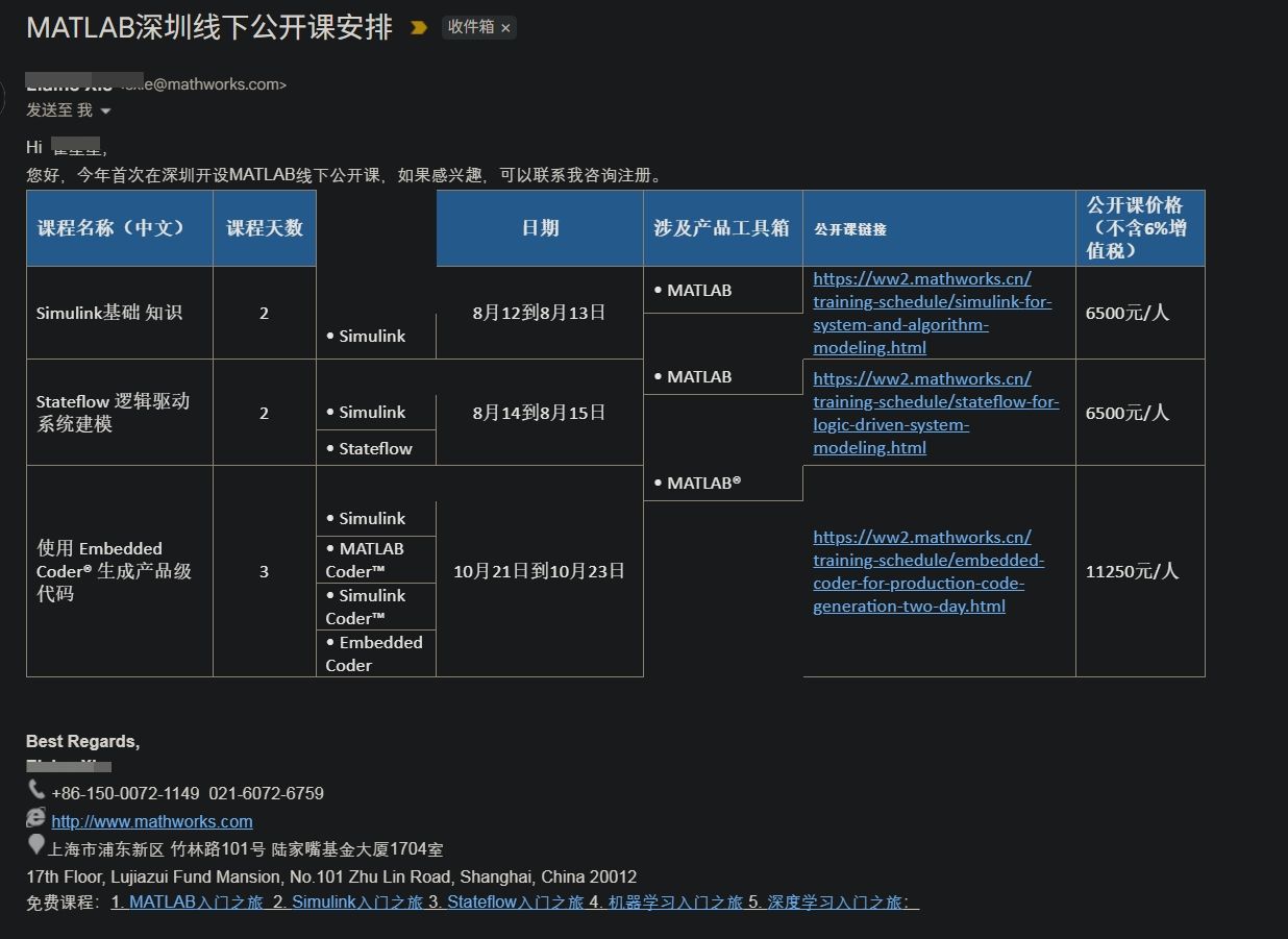
I’d love to hear your thoughts and start a discussion on this!
I am thrilled python interoperability now seems to work for me with my APPLE M1 MacBookPro and MATLAB V2025a. The available instructions are still, shall we say, cryptic. Here is a summary of my interaction with GPT 4o to get this to work.
===========================================================
MATLAB R2025a + Python (Astropy) Integration on Apple Silicon (M1/M2/M3 Macs)
===========================================================
Author: D. Carlsmith, documented with ChatGPT
Last updated: July 2025
This guide provides full instructions, gotchas, and workarounds to run Python 3.10 with MATLAB R2025a (Apple Silicon/macOS) using native ARM64 Python and calling modules like Astropy, Numpy, etc. from within MATLAB.
===========================================================
Overview
===========================================================
- MATLAB R2025a on Apple Silicon (M1/M2/M3) runs as "maca64" (native ARM64).
- To call Python from MATLAB, the Python interpreter must match that architecture (ARM64).
- Using Intel Python (x86_64) with native MATLAB WILL NOT WORK.
- The cleanest solution: use Miniforge3 (Conda-forge's lightweight ARM64 distribution).
===========================================================
1. Install Miniforge3 (ARM64-native Conda)
===========================================================
In Terminal, run:
curl -LO https://github.com/conda-forge/miniforge/releases/latest/download/Miniforge3-MacOSX-arm64.sh
bash Miniforge3-MacOSX-arm64.sh
Follow prompts:
- Press ENTER to scroll through license.
- Type "yes" when asked to accept the license.
- Press ENTER to accept the default install location: ~/miniforge3
- When asked:
Do you wish to update your shell profile to automatically initialize conda? [yes|no]
Type: yes
===========================================================
2. Restart Terminal and Create a Python Environment for MATLAB
===========================================================
Run the following:
conda create -n matlab python=3.10 astropy numpy -y
conda activate matlab
Verify the Python path:
which python
Expected output:
/Users/YOURNAME/miniforge3/envs/matlab/bin/python
===========================================================
3. Verify Python + Astropy From Terminal
===========================================================
Run:
python -c "import astropy; print(astropy.__version__)"
Expected output:
6.x.x (or similar)
===========================================================
4. Configure MATLAB to Use This Python
===========================================================
In MATLAB R2025a (Apple Silicon):
clear classes
pyenv('Version', '/Users/YOURNAME/miniforge3/envs/matlab/bin/python')
py.sys.version
You should see the Python version printed (e.g. 3.10.18). No error means it's working.
===========================================================
5. Gotchas and Their Solutions
===========================================================
❌ Error: Python API functions are not available
→ Cause: Wrong architecture or broken .dylib
→ Fix: Use Miniforge ARM64 Python. DO NOT use Intel Anaconda.
❌ Error: Invalid text character (↑ points at __version__)
→ Cause: MATLAB can’t parse double underscores typed or pasted
→ Fix: Use: py.getattr(module, '__version__')
❌ Error: Unrecognized method 'separation' or 'sec'
→ Cause: MATLAB can't reflect dynamic Python methods
→ Fix: Use: py.getattr(obj, 'method')(args)
===========================================================
6. Run Full Verification in MATLAB
===========================================================
Paste this into MATLAB:
% Set environment
clear classes
pyenv('Version', '/Users/YOURNAME/miniforge3/envs/matlab/bin/python');
% Import modules
coords = py.importlib.import_module('astropy.coordinates');
time_mod = py.importlib.import_module('astropy.time');
table_mod = py.importlib.import_module('astropy.table');
% Astropy version
ver = char(py.getattr(py.importlib.import_module('astropy'), '__version__'));
disp(['Astropy version: ', ver]);
% SkyCoord angular separation
c1 = coords.SkyCoord('10h21m00s', '+41d12m00s', pyargs('frame', 'icrs'));
c2 = coords.SkyCoord('10h22m00s', '+41d15m00s', pyargs('frame', 'icrs'));
sep_fn = py.getattr(c1, 'separation');
sep = sep_fn(c2);
arcsec = double(sep.to('arcsec').value);
fprintf('Angular separation = %.3f arcsec\n', arcsec);
% Time difference in seconds
Time = time_mod.Time;
t1 = Time('2025-01-01T00:00:00', pyargs('format','isot','scale','utc'));
t2 = Time('2025-01-02T00:00:00', pyargs('format','isot','scale','utc'));
dt = py.getattr(t2, '__sub__')(t1);
seconds = double(py.getattr(dt, 'sec'));
fprintf('Time difference = %.0f seconds\n', seconds);
% Astropy table display
tbl = table_mod.Table(pyargs('names', {'a','b'}, 'dtype', {'int','float'}));
tbl.add_row({1, 2.5});
tbl.add_row({2, 3.7});
disp(tbl);
===========================================================
7. Optional: Automatically Configure Python in startup.m
===========================================================
To avoid calling pyenv() every time, edit your MATLAB startup:
edit startup.m
Add:
try
pyenv('Version', '/Users/YOURNAME/miniforge3/envs/matlab/bin/python');
catch
warning("Python already loaded.");
end
===========================================================
8. Final Notes
===========================================================
- This setup avoids all architecture mismatches.
- It uses a clean, minimal ARM64 Python that integrates seamlessly with MATLAB.
- Do not mix Anaconda (Intel) with Apple Silicon MATLAB.
- Use py.getattr for any Python attribute containing underscores or that MATLAB can't resolve.
You can now run NumPy, Astropy, Pandas, Astroquery, Matplotlib, and more directly from MATLAB.
===========================================================
One of MATLAB's strengths is how easy it is to document a custom function/class. The first continuous comment block is automatially displayed by the help and doc functions, with some neat automatic formatting. For example:
% myFunc My example function
%
% This function does not do anything yet, but one day will be great. For
% example, you will be able to type:
% out=myFunc(in1,in2);
% and something cool will happen.
%
% See also otherFunc
function varargout=myFunc(varargin)
% actual code
end
will have a link to the documentation for "otherFunc", assuming that file exists. Class documentation is nicely broken up into a header (with "See also" support) followed by a property and method summary.
All the above works great with one big exception: apart from highlighting uses of the file's name, there is no way to display anything but pure text. No Markdown, no LateX, and so forth. It is possible to sneak an HTML link into the comment block, calling a MATLAB command that can display a live script with fancy formatting. I have done this in the past, although it can be a little tricky for files inside a package/namespace (folders beginning with '+').
I can envision a system where fancy documentation would be buried inside an "example" subfolder where "myFunc.m" is located. Invoking "showExample myFunc", where "showExample" is a to-be-written utility, would look for a live script inside the appropriate subfolder, make a local copy for the user to tinker with, and then display that local copy in the MATLAB editor. Since the actual function function and its example woulld obviously inside a Git repository, text-based live scripts would be used instead of an *.mlx file.
Again, this all works fine on its fine on its own, but it would be very difficult to replicate the "See also" capability or the other features of the standard doc function. So what are we to do? Is there a clever way to add another block to a standard comment block "See examples" that would automatically detect scripts in a subfolder of function/class being queried?
I know there is a way to incorporate custom documentation into MATLAB help system. This is much too cumbersome for my purposes, where many functions/classes are being added/edited all the time. The existing doc system covers maybe 80% of my needs, but sometimes a little math (LaTeX) would go a long way on explaining how things work.
Are you a dark mode enthusiast or are you curious about how it’s shaping MATLAB graphics? Check out the latest article in the MATLAB Graphics and App Building blog.
🔹 User Insights: find out how user surveys influenced the development of graphics themes
🔹 Learn three ways to switch between light and dark themes for figures
🔹 Understand how custom and default colors behave across themes
🔹 Download a handy cheat sheet for working with themes in your graphics and apps.
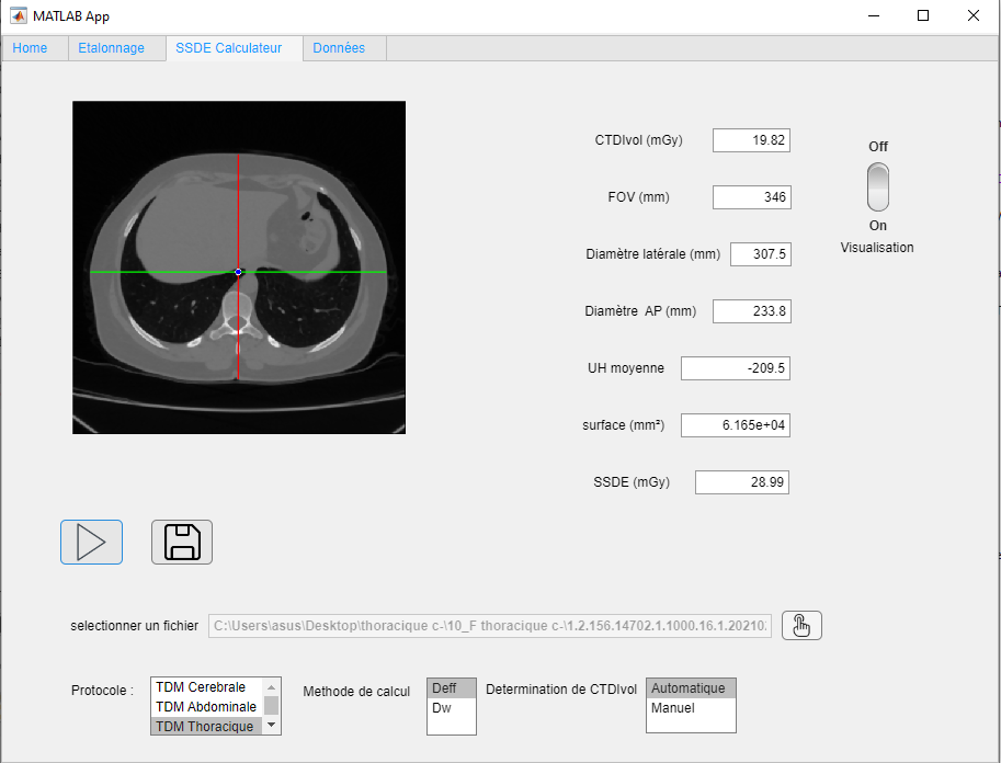
automatisation du calcul du SSDE(Size Specific Dose Estimate )