搜索
What is a rough number? What can they be used for? Today I'll take you down a journey into the land of prime numbers (in MATLAB). But remember that a journey is not always about your destination, but about what you learn along the way. And so, while this will be all about primes, and specifically large primes, before we get there we need some background. That will start with rough numbers.
Rough numbers are what I would describe as wannabe primes. Almost primes, and even sometimes prime, but often not prime. They could've been prime, but may not quite make it to the top. (If you are thinking of Marlon Brando here, telling us he "could've been a contender", you are on the right track.)
Mathematically, we could call a number k-rough if it is evenly divisible by no prime smaller than k. (Some authors will use the term k-rough to denote a number where the smallest prime factor is GREATER than k. The difference here is a minor one, and inconsequential for my purposes.) And there are also smooth numbers, numerical antagonists to the rough ones, those numbers with only small prime factors. They are not relevant to the topic today, even though smooth numbers are terribly valuable tools in mathematics. Please forward my apologies to the smooth numbers.
Have you seen rough numbers in use before? Probably so, at least if you ever learned about the sieve of Eratosthenes for prime numbers, though probably the concept of roughness was never explicitly discussed at the time. The sieve is simple. Suppose you wanted a list of all primes less than 100? (Without using the primes function itself.)
% simple sieve of Eratosthenes
Nmax = 100;
N = true(1,Nmax); % A boolean vector which when done, will indicate primes
N(1) = false; % 1 is not a prime by definition
nextP = find(N,1,'first'); % the first prime is 2
while nextP <= sqrt(Nmax)
% flag multiples of nextP as not prime
N(nextP*nextP:nextP:end) = false;
% find the first element after nextP that remains true
nextP = nextP + find(N(nextP+1:end),1,'first');
end
primeList = find(N)
Indeed, that is the set of all 25 primes not exceeding 100. If you think about how the sieve worked, it first found 2 is prime. Then it discarded all integer multiples of 2. The first element after 2 that remains as true is 3. 3 is of course the second prime. At each pass through the loop, the true elements that remain correspond to numbers which are becoming more and more rough. By the time we have eliminated all multiples of 2, 3, 5, and finally 7, everything else that remains below 100 must be prime! The next prime on the list we would find is 11, but we have already removed all multiples of 11 that do not exceed 100, since 11^2=121. For example, 77 is 11*7, but we already removed it, because 77 is a multiple of 7.
Such a simple sieve to find primes is great for small primes. However is not remotely useful in terms of finding primes with many thousands or even millions of decimal digits. And that is where I want to go, eventually. So how might we use roughness in a useful way? You can think of roughness as a way to increase the relative density of primes. That is, all primes are rough numbers. In fact, they are maximally rough. But not all rough numbers are primes. We might think of roughness as a necessary, but not sufficient condition to be prime.
How many primes lie in the interval [1e6,2e6]?
numel(primes(2e6)) - numel(primes(1e6))
There are 70435 primes greater than 1e6, but less than 2e6. Given there are 1 million natural numbers in that set, roughly 7% of those numbers were prime. Next, how many 100-rough numbers lie in that same interval?
N = (1e6:2e6)';
roughInd = all(mod(N,primes(100)) > 0,2);
sum(roughInd)
That is, there are 120571 100-rough numbers in that interval, but all those 70435 primes form a subset of the 100-rough numbers. What does this tell us? Of the 1 million numbers in that interval, approximately 12% of them were 100-rough, but 58% of the rough set were prime.
The point being, if we can efficiently identify a number as being rough, then we can substantially increase the chance it is also prime. Roughness in this sense is a prime densifier. (Is that even a word? It is now.) If we can reduce the number of times we need to perform an explicit isprime test, that will gain greatly because a direct test for primality is often quite costly in CPU time, at least on really large numbers.
In my next post, I'll show some ways we can employ rough numbers to look for some large primes.
Do you boast about the energy savings you racking up by using dark mode while stashing your energy bill savings away for an exotic vacation🌴🥥? Well, hold onto your sun hats and flipflops!
A recent study presented at the 1st Internaltional Workshop on Low Carbon Computing suggests that you may be burning more ⚡energy⚡ with your slick dark displays 💻[1].
In a 2x2 factorial design, ten participants viewed a webpage in dark and light modes in both dim and lit settings using an LCD monitor with 16 brightness levels.
- 80% of participants increased the monitor's brightness in dark mode [2]
- This occurred in both lit and dim rooms
- Dark mode did not reduce power draw but increasing monitor brightness did.
The color pixels in an LCD monitor still draw voltage when the screen is black, which is why the monitor looks gray when displaying a pure black background in a dark room. OLED monitors, on the other hand, are capable of turning off pixels that represent pure black and therefore have the potential to save energy with dark mode. A 2021 Purdue study estimates a 3%-9% energy savings with dark mode on OLED monitors using auto-brightness [3]. However, outside of gaming, OLED monitors have a very small market share and still account for less than 25% within the gaming world.
Any MATLAB users out there with OLED monitors? How are you going to spend your mad cash savings when you start using MATLAB's upcoming dark theme?
- BBC study: https://www.sicsa.ac.uk/wp-content/uploads/2024/11/LOCO2024_paper_12.pdf
- BBC blog article https://www.bbc.co.uk/rd/articles/2025-01-sustainability-web-energy-consumption
- 2021 Purdue https://dl.acm.org/doi/abs/10.1145/3458864.3467682
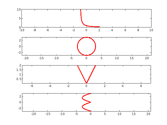
tiledlayout(4,1);
% Plot "L" (y = 1/(x+1), for x > -1)
x = linspace(-0.9, 2, 100); % Avoid x = -1 (undefined)
y =1 ./ (x+1) ;
nexttile;
plot(x, y, 'r', 'LineWidth', 2);
xlim([-10,10])
% Plot "O" (x^2 + y^2 = 9)
theta = linspace(0, 2*pi, 100);
x = 3 * cos(theta);
y = 3 * sin(theta);
nexttile;
plot(x, y, 'r', 'LineWidth', 2);
axis equal;
% Plot "V" (y = -2|x|)
x = linspace(-1, 1, 100);
y = 2 * abs(x);
nexttile;
plot(x, y, 'r', 'LineWidth', 2);
axis equal;
% Plot "E" (x = -3 |sin(y)|)
y = linspace(-pi, pi, 100);
x = -3 * abs(sin(y));
nexttile;
plot(x, y, 'r', 'LineWidth', 2);
axis equal;
I've been trying this problem a lot of time and i don't understand why my solution doesnt't work.
In 4 tests i get the error Assertion failed but when i run the code myself i get the diag and antidiag correctly.
function [diag_elements, antidg_elements] = your_fcn_name(x)
[m, n] = size(x);
% Inicializar los vectores de la diagonal y la anti-diagonal
diag_elements = zeros(1, min(m, n));
antidg_elements = zeros(1, min(m, n));
% Extraer los elementos de la diagonal
for i = 1:min(m, n)
diag_elements(i) = x(i, i);
end
% Extraer los elementos de la anti-diagonal
for i = 1:min(m, n)
antidg_elements(i) = x(m-i+1, i);
end
end
On 27th February María Elena Gavilán Alfonso and I will be giving an online seminar that has been a while in the making. We'll be covering MATLAB with Jupyter, Visual Studio Code, Python, Git and GitHub, how to make your MATLAB projects available to the world (no installation required!) and much much more.
Sign up (it's free!) at MATLAB Without Borders: Connecting your Projects with Python and other Open-Source Tools - MATLAB & Simulink

Of course
62.5%
I never tried
37.5%
16 个投票
Check out the result of "emoji matrix" multiplication below.
- vector multiply vector:
a = ["😁","😁","😁"]
b = ["😂";
"😂"
"😂"]
c = a*b
d = b*a
- matrix multiply matrix:
matrix1 = [
"😀", "😃";
"😄", "😁"]
matrix2 = [
"😆", "😅";
"😂", "🤣"]
resutl = matrix1*matrix2
enjoy yourself!
I am looking for a Simulink tutor to help me with Reinforcement Learning Agent integration. If you work for MathWorks, I am willing to pay $30/hr. I am working on a passion project, ready to start ASAP. DM me if you're interested.
Bitte um Hilfe beim Kauf
I love it all
45%
Love the first snowfall only
15%
Hate it
17.5%
It doesn't snow where I live
22.5%
40 个投票
Since May 2023, MathWorks officially introduced the new Community API(MATLAB Central Interface for MATLAB), which supports both MATLAB and Node.js languages, allowing users to programmatically access data from MATLAB Answers, File Exchange, Blogs, Cody, Highlights, and Contests.
I’m curious about what interesting things people generally do with this API. Could you share some of your successful or interesting experiences? For example, retrieving popular Q&A topics within a certain time frame through the API and displaying them in a chart.
If you have any specific examples or ideas in mind, feel free to share!
For Valentine's day this year I tried to do something a little more than just the usual 'Here's some MATLAB code that draws a picture of a heart' and focus on how to share MATLAB code. TL;DR, here's my advice
- Put the code on GitHub. (Allows people to access and collaborate on your code)
- Set up 'Open in MATLAB Online' in your GitHub repo (Allows people to easily run it)
I used code by @Zhaoxu Liu / slandarer and others to demonstrate. I think that those two steps are the most impactful in that they get you from zero to one but If I were to offer some more advice for research code it would be
3. Connect the GitHub repo to File Exchange (Allows MATLAB users to easily find it in-product).
4. Get a Digitial Object Identifier (DOI) using something like Zenodo. (Allows people to more easily cite your code)
There is still a lot more you can do of course but if everyone did this for any MATLAB code relating to a research paper, we'd be in a better place I think.
Here's the article: On love and research software: Sharing code with your Valentine » The MATLAB Blog - MATLAB & Simulink
What do you think?
On my computers, this bit of code produces an error whose cause I have pinpointed,
load tstcase
ycp=lsqlin(I, y, Aineq, bineq);
Error using parseOptions
Too many output arguments.
Error in lsqlin (line 170)
[options, optimgetFlag] = parseOptions(options, 'lsqlin', defaultopt);
^^^^^^^^^^^^^^^^^^^^^^^^^^^^^^^^^^^^^^^^^^^
The reason for the error is seemingly because, in recent Matlab, lsqlin now depends on a utility function parseOptions, which is shadowed by one of my personal functions sharing the same name:
C:\Users\MWJ12\Documents\mwjtree\misc\parseOptions.m
C:\Program Files\MATLAB\R2024b\toolbox\shared\optimlib\parseOptions.m % Shadowed
The MathWorks-supplied version of parseOptions is undocumented, and so is seemingly not meant for use outside of MathWorks. Shouldn't it be standard MathWorks practice to put these utilities in a private\ folder where they cannot conflict with user-supplied functions of the same name?
It is going to be an enormous headache for me to now go and rename all calls to my version of parseOptions. It is a function I have been using for a long time and permeates my code.
General observations on practical implementation issues regarding add-on versioning
I am making updates to one of my File Exchange add-ons, and the updates will require an updated version of another add-on. The state of versioning for add-ons seems to be a bit of a mess.
First, there are several sources of truth for an add-on’s version:
- The GitHub release version, which gets mirrored to the File Exchange version
- The ToolboxVersion property of toolboxOptions (for an add-on packaged as a toolbox)
- The version in the Contents.m file (if there is one)
Then, there is the question of how to check the version of an installed add-on. You can call matlab.addon.installedAddons, which returns a table. Then you need to inspect the table to see if a particular add-on is present, if it is enabled, and get the version number.
If you can get the version number this way, then you need some code to compare two semantic version numbers (of the form “3.1.4”). I’m not aware of a documented MATLAB function for this. The verLessThan function takes a toolbox name and a version; it doesn’t help you with comparing two versions.
If add-on files were downloaded directly and added to the MATLAB search path manually, instead of using the .mtlbx installer file, the add-on won’t be listed in the table returned by matlab.addon.installedAddon. You’d have to call ver to get the version number from the Contents.m file (if there is one).
Frankly, I don’t want to write any of this code. It would take too long, be challenging to test, and likely be fragile.
Instead, I think I will write some sort of “capabilities” utility function for the add-on. This function will be used to query the presence of needed capabilities. There will still be a slight coding hassle—the client add-on will need to call the capabilities utility function in a try-catch, because earlier versions of the add-on will not have that utility function.
I also posted this over at Harmonic Notes
I got thoroughly nerd-sniped by this xkcd, leading me to wonder if you can use MATLAB to figure out the dice roll for any given (rational) probability. Well, obviously you can. The question is how. Answer: lots of permutation calculations and convolutions.
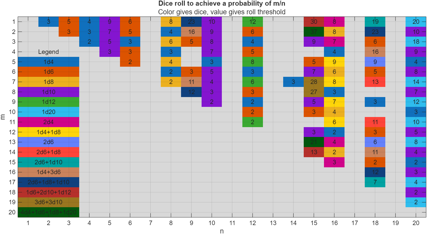
In the original xkcd, the situation described by the player has a probability of 2/9. Looking up the plot, row 2 column 9, shows that you need 16 or greater on (from the legend) 1d4+3d6, just as claimed.
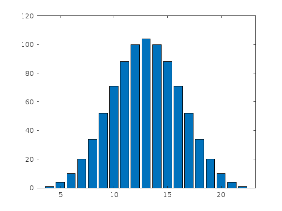
If you missed the bit about convolutions, this is a super-neat trick
[v,c] = dicedist([4 6 6 6]);
bar(v,c)
% Probability distribution of dice given by d
function [vals,counts] = dicedist(d)
% d is a vector of number of sides
n = numel(d); % number of dice
% Use convolution to count the number of ways to get each roll value
counts = 1;
for k = 1:n
counts = conv(counts,ones(1,d(k)));
end
% Possible values range from n to sum(d)
maxtot = sum(d);
vals = n:maxtot;
end
My following code works running Matlab 2024b for all test cases. However, 3 of 7 tests fail (#1, #4, & #5) the QWERTY Shift Encoder problem. Any ideas what I am missing?
Thanks in advance.
keyboardMap1 = {'qwertyuiop[;'; 'asdfghjkl;'; 'zxcvbnm,'};
keyboardMap2 = {'QWERTYUIOP{'; 'ASDFGHJKL:'; 'ZXCVBNM<'};
if length(s) == 0
se = s;
end
for i = 1:length(s)
if double(s(i)) >= 65 && s(i) <= 90
row = 1;
col = 1;
while ~strcmp(s(i), keyboardMap2{row}(col))
if col < length(keyboardMap2{row})
col = col + 1;
else
row = row + 1;
col = 1;
end
end
se(i) = keyboardMap2{row}(col + 1);
elseif double(s(i)) >= 97 && s(i) <= 122
row = 1;
col = 1;
while ~strcmp(s(i), keyboardMap1{row}(col))
if col < length(keyboardMap1{row})
col = col + 1;
else
row = row + 1;
col = 1;
end
end
se(i) = keyboardMap1{row}(col + 1);
else
se(i) = s(i);
end
% if ~(s(i) = 65 && s(i) <= 90) && ~(s(i) >= 97 && s(i) <= 122)
% se(i) = s(i);
% end
end
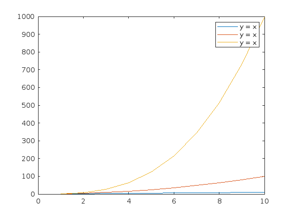
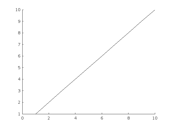
Currently, according to the official documentation, "DisplayName" only supports character vectors or single scalar string as input. For example, when plotting three variables simultaneously, if I use a single scalar string as input, the legend labels will all be the same. To have different labels, I need to specify them separately using the legend function with label1, label2, label3.
Here's an example illustrating the issue:
x = (1:10)';
y1 = x;
y2 = x.^2;
y3 = x.^3;
% Plotting with a string scalar for DisplayName
figure;
plot(x, [y1,y2,y3], DisplayName="y = x");
legend;
% To have different labels, I need to use the legend function separately
figure;
plot(x, [y1,y2,y3], DisplayName=["y = x","y = x^2","y=x^3"]);
% legend("y = x","y = x^2","y=x^3");
Three former MathWorks employees, Steve Wilcockson, David Bergstein, and Gareth Thomas, joined the ArrayCast pod cast to discuss their work on array based languages. At the end of the episode, Steve says,
> It's a little known fact about MATLAB. There's this thing, Gareth has talked about the community. One of the things MATLAB did very, very early was built the MATLAB community, the so-called MATLAB File Exchange, which came about in the early 2000s. And it was where people would share code sets, M files, et cetera. This was long before GitHub came around. This was well ahead of its time. And I think there are other places too, where MATLAB has delivered cultural benefits over and above the kind of core programming and mathematical capabilities too. So, you know, MATLAB Central, File Exchange, very much saw the future.
Listen here: The ArrayCast, Episode 79, May 10, 2024.
This topic is for discussing highlights to the current R2025a Pre-release.
So you've downloaded the R2025a pre-release, tried Dark mode and are wondering what else is new. A lot! A lot is new!
One thing I am particularly happy about is the fact that Apple Accelerate is now the default BLAS on Apple Silicon machines. Check it out by doing
>> version -blas
ans =
'Apple Accelerate BLAS (ILP64)'
If you compare this to R2024b that is using OpenBLAS you'll see some dramatic speed-ups in some areas. For example, I saw up to 3.7x speed-up for matrix-matrix multiplication on my M2 Mabook Pro and 2x faster LU factorisation.
Details regarding my experiments are in this blog post Life in the fast lane: Making MATLAB even faster on Apple Silicon with Apple Accelerate » The MATLAB Blog - MATLAB & Simulink . Back then you had to to some trickery to switch to Apple Accelerate, now its the default.