Results for

1. Use the new exportapp function to capture an image of your app|uifigure
2. MATLAB's getframe now supports apps & uifigures
3. Review: How to get the handle to an app figure

Use the new exportapp function to capture an image of your app|uifigure

Imagine these scenarios:

• Your app contains several adjustable parameters that update an embedded plot and you'd like to remember the values of each app component so that you can recreate the plot with the same dataset
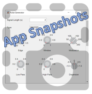
• You're constructing a manual for your app and would like to include images of your app
• You're app contains a process that automatically updates regularly and you'd like to store periodic snapshots of your app.

As of MATLABs R2020b release , we no longer must rely on 3rd party software to record an image of an app or uifigure.

exportapp(fig,filename) saves an image (JPEG | PNG | TIFF | PDF) of a uifigure ( fig) with the specified file name or full file path ( filename). MATLAB's documentation includes an example of how to add an [Export] button to an app that allows the user to select a path, filename, and extension for their exported image.

Here's another example that merely saves the image as a PDF to the app's main folder.

1. Add a button to the app and assign a ButtonPushed callback function to the button. This one also assigns an icon to the button in the form of an svg file.

2. Define the callback function to name the image after the app's name and include a datetime stamp. The image will be saved to the app's main folder.

% Button pushed function: SnapshotButton
function SnapshotButtonPushed(app, ~) 
    % create filename containing the app's figure name (spaces removed)
    % and a datetime stamp in format yymmdd_hhmmss
    filename = sprintf('%s_%s.pdf',regexprep(app.MyApp.Name,' +',''), datestr(now(),'yymmdd_HHMMSS'));
    % Get the app's path
    filepath = fileparts(which([mfilename,'.mlapp']));
    % Store snapshot
    exportapp(app.MyApp, fullfile(filepath,filename))
end

Matlab's getframe now supports apps & uifigures

getframe(h) captures images of axes or a uifigure as a structure containing the image data which defines a movie frame. This function has been around for a while but as of r2020b , it now supports uifigures. By capturing consecutive frames, you can create a movie that can be played back within a Matlab figure (using movie ) or as an AVI file (using VideoWriter ). This is useful when demonstrating the effects of changes to app components.

The general steps to recording a process within an app as a movie are,

1. Add a button or some other event to your app that can invoke the frame recording process.

2. Animation is typically controlled by a loop with n iterations. Preallocate the structure array that will store the outputs to getframe. The example below stores the outputs within the app so that they are available by other functions within the app. That will require you to define the variable as a property in the app.

% nFrames is the number of iterations that will be recorded.
% recordedFrames is defined as a private property within the app
app.recordedFrames(1:nFrames) = struct('cdata',[],'colormap',[]);

3. Call getframe from within the loop that controls the animation. If you're using VideoWriter to create an AVI file, you'll also do that here (not shown, but see an example in the documentation ).

% app.myAppUIFigure: the app's figure handle
% getframe() also accepts axis handles
for i = 1:nFrames

      ... % code that updates the app for the next frame

      app.recordedFrames(i) = getframe(app.myAppUIFigure);
  end

4. Now the frame data are stored in app.recordedFrames and can be accessed from anywhere within the app. To play them back as a movie,

movie(app.recordedFrames) 
% or 
movie(app.recordedFrames, n) % to play the movie n-times
movie(app.recordedFrames, n, fps) % to specify the number of frames per second

To demonstrate this, I adapted a copy of Matlab's built-in PulseGenerator.mlapp by adding

• a record button
• a record status lamp with frame counter
• a playback button
• a function that animates the effects of the Edge Knob

Recording process (The GIF is a lot faster than realtime and only shows part of the recording) (Open the image in a new window or see the attached Live Script for a clearer image).

Playback process (Open the image in a new window or see the attached Live Script for a clearer image.)

Review: How to get the handle to an app figure

To use either of these functions outside of app designer, you'll need to access the App's figure handle. By default, the HandleVisibility property of uifigures is set to off preventing the use of gcf to retrieve the figure handle. Here are 4 ways to access the app's figure handle from outside of the app.

1. Store the app's handle when opening the app.

app = myApp;
% Get the figure handle
figureHandle = app.myAppUIFigure;

2. Search for the figure handle using the app's name, tag, or any other unique property value

allfigs = findall(0, 'Type', 'figure'); % handle to all existing figures
figureHandle = findall(allfigs, 'Name', 'MyApp', 'Tag', 'MyUniqueTagName');

3. Change the HandleVisibility property to on or callback so that the figure handle is accessible by gcf anywhere or from within callback functions. This can be changed programmatically or from within the app designer component browser. Note, this is not recommended since any function that uses gcf such as axes(), clf(), etc can now access your app!.

4. If the app's figure handle is needed within a callback function external to the app, you could pass the app's figure handle in as an input variable or you could use gcbf() even if the HandleVisibility is off.

See a complete list of changes to the PulseGenerator app in the attached Live Script file to recreate the app.

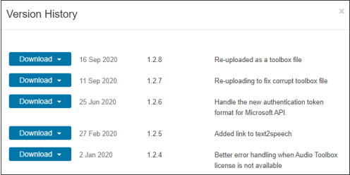
File Exchange now offers the ability to download/restore previous versions of community contributed files. It's often a good practice to always update your software to the latest version, however there are times when this isn't always helpful. Sometimes a software update can break or alter something you've been relying on, in these cases you'll want to stick with the version that's working for you. This is why we've added the ability to download previous versions in File Exchange.

Using Version History

Navigate to any community member file and then click the View Version History link that appears above the Download button. This will show you a list of the previous versions contributed by the submission author. Each version will have a corresponding download button, date, version number, and a description of the changes made for that update.

Let us know what you think about this new feature by replying below.

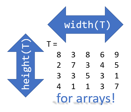
Prior to r2020b the height (number of rows) and width (number of columns) of an array or table can be determined by the size function,

array = rand(102, 16);

% Method 1
[dimensions] = size(array);
h = dimensions(1);
w = dimensions(2);

% Method 2
[h, w] = size(array); %#ok<*ASGLU>
% or
[h, ~] = size(array);
[~, w] = size(array);

% Method 3
h = size(array,1);
w = size(array,2);

In r2013b, the height(T) and width(T) functions were introduced to return the size of single dimensions for tables and timetables.

Starting in r2020b, height() and width() can be applied to arrays as an alternative to the size() function.

Continuing from the section above,

h = height(array)
% h =  102

w = width(array)
% w =  16

height() and width() can also be applied to multidimensional arrays including cell and structure arrays

mdarray = rand(4,3,20);
h = height(mdarray)
% h =  4

w = width(mdarray)
% w =  3

The expanded support of the height() and width() functions means,

1. when reading code, you can no longer assume the variable T in height(T) or width(T) refers to a table or timetable
2. greater flexibility in expressions such as the these, below

% C is a 1x4 cell array containing 4 matrices with different dimensions
rng('default')
C = {rand(5,2), rand(2,3), rand(3,4), rand(1,1)};
celldisp(C)

% C{1} =
%       0.81472      0.09754
%       0.90579       0.2785
%       0.12699      0.54688
%       0.91338      0.95751
%       0.63236      0.96489
% C{2} =
%       0.15761      0.95717      0.80028
%       0.97059      0.48538      0.14189
% C{3} =
%       0.42176      0.95949      0.84913      0.75774
%       0.91574      0.65574      0.93399      0.74313
%       0.79221     0.035712      0.67874      0.39223
% C{4} =
%       0.65548

What's the max number of rows in C?

maxRows1 = max(cellfun(@height,C))         % using height()
% maxRows1 =  5;

maxRows2 = max(cellfun(@(x)size(x,1),C))   % using size()
% maxRows2 =  5; 

What's the total number of columns in C?

totCols1 = sum(cellfun(@width,C))          % using width()
%totCols1 =  10

totCols2 = sum(cellfun(@(x)size(x,2),C))   % using size(x,2)
% totCols2 =  10

Attached is a live script containing the content of this post.

We are excited to announce that Cody Contest 2020 starts today! Again, the rule is simple - solve any problem and rate its difficulty. If you have any question, please visit our FAQs page first. Want to know your ranking? Check out the contest leaderboard .

Happy problem-solving! We hope you are a winner.

Please join Loren Shure for her live sessions on the MATLAB YouTube channel starting October 1st and continuing through November 19th. You know Loren from her popular blog Loren on the Art of MATLAB.

Solve coding problems. Improve MATLAB skills. Have fun. See details and register .

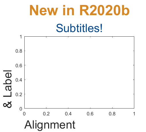
Add a subtitle

Multi-lined titles have been supported for a long time but starting in r2020b, you can add a subtitle with its own independent properties to a plot in two easy ways.

1. Use the new subtitle function: s=subtitle('mySubtitle')
2. Use the new second argument to the title function: [t,s]=title('myTitle','mySubtitle')

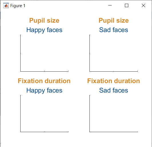
figure()
tiledlayout(2,2)

% Method 1
ax(1) = nexttile;
th(1) = title('Pupil size'); 
sh(1) = subtitle('Happy faces');

ax(2) = nexttile;
th(2) = title('Pupil size'); 
sh(2) = subtitle('Sad faces');

% Method 2
ax(3) = nexttile;
[th(3), sh(3)] = title('Fixation duration', 'Happy faces'); 

ax(4) = nexttile;
[th(4), sh(4)] = title('Fixation duration', 'Sad faces'); 

set(ax, 'xticklabel', [], 'yticklabel', [],'xlim',[0,1],'ylim',[0,1])

% Set all title colors to orange and subtitles colors to purple.
set(th, 'Color', [0.84314, 0.53333, 0.1451])
set(sh, 'Color', [0, 0.27843, 0.56078])

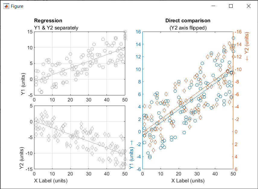
Control title/Label alignment

Title and axis label positions can be changed via their Position, VerticalAlignment and HorizontalAlignment properties but this is usually clumsy and leads to other problems when trying to align the title or labels with an axis edge. For example, when the position units are set to 'data' and the axis limits change, the corresponding axis label will change position relative to the axis edges. If units are normalized and the axis position or size changes, the corresponding label will no longer maintain its relative position to the axis, and that's assuming the normalized position was computed correctly in the first place.

Starting in r2020b, title and axis label alignment can be set to center|left|right, relative to the axis edges.

• TitleHorizontalAlignment is a property of the axis: h.TitleHorizontalAlignment='left';
• LabelHorizontalAlignment is a property of the ruler object that defines the x | y | z axis: h.XAxis.LabelHorizontalAlignment='left';

% Create data
x = randi(50,1,100)'; 
y = x.*[.2, -.2] + (rand(numel(x),2)-.5)*10; 
gray = [.65 .65 .65];

% Plot comparison between columns of y
figure()
tiledlayout(2,2,'TileSpacing','none')
ax(1) = nexttile(1);
plot(x, y(:,1), 'o', 'color', gray)
lsline
ylabel('Y1 (units)')
title('Regression','Y1 & Y2 separately')

ax(2) = nexttile(3);
plot(x, y(:,2), 'd', 'color', gray)
lsline
xlabel('X Label (units)')
ylabel('Y2 (units)')
grid(ax, 'on')
linkaxes(ax, 'x')

%  Move title and labels leftward
set(ax, 'TitleHorizontalAlignment', 'left')
set([ax.XAxis], 'LabelHorizontalAlignment', 'left')
set([ax.YAxis], 'LabelHorizontalAlignment', 'left')

% Combine the two comparisons into plot and flip the second 
% y-axis so trend are in the same direction
ax(3) = nexttile([2,1]);
yyaxis('left')
plot(x, y(:,1), 'o')
ylim([-6,16])
lsline
xlabel('X Label (units)')
ylabel('Y1 (units) \rightarrow')

yyaxis('right')
plot(x, y(:,2), 'd')
ylim([-16,6])
lsline
ylabel('\leftarrow Y2 (units)')
title('Direct comparison','(Y2 axis flipped)')
set(ax(3),  'YDir','Reverse')

% Align the ylabels with the minimum axis limit to emphasize the
% directions of each axis. Keep the title and xlabel centered
ax(3).YAxis(1).LabelHorizontalAlignment = 'left';
ax(3).YAxis(2).LabelHorizontalAlignment = 'right';
ax(3).TitleHorizontalAlignment = 'Center';       % not needed; default value.
ax(3).XAxis.LabelHorizontalAlignment = 'Center'; % not needed; default value.

Below are some FAQs for the Cody contest 2020. If you have any additional questions, ask your questions by replying to this post. We will keep updating the FAQs.

Q1: If I rate a problem I solved before the contest, will I still get a raffle ticket?

A: Yes. You can rate any problem you have solved, whether it was before or during the contest period.

Q2: When will I receive the contest badges that I've earned?

A: All badges will be awarded after the contest ends.

Q3: How do I know if I’m the raffle winner?

A: If you are a winner, we will contact you to get your name and mailing address. You can find the list of winners on the Cody contest page .

Q4: When will I receive my T-shirt or hat?

A: You will typically receive your prize within a few weeks. It might take longer for international shipping.

Q5: I'm new to Cody. If I have some questions about using Cody, how can I get help?

A: You can ask your question by replying this post. Other community users might help you and we will also monitor the threads. You might also find answers here .

Q6: What do I do if I have a question about a specific problem?

A: If the problem description is unclear, the test suite is broken, or similar concerns arise, post your question(s) as a comment on the specific problem page. If you are having a hard time solving a problem, you can post a comment to your solution attempt (after submitting it). However, do not ask other people to solve problems for you.

Q7: If I find a bug or notice someone is cheating/spamming during the contest, how can I report it?

A: Use Web Site Feedback . Select "MATLAB Central" from the category list.

Q8: Why can't I rate a problem?

A: To rate a problem, you must solve that problem first and have at least 50 total points.

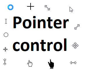
Starting in r2020a , you can change the mouse pointer symbol in apps and uifigures.

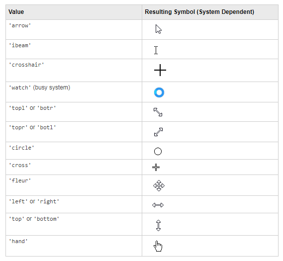
The Pointer property of a figure defines the cursor’s default pointer symbol within the figure. You can also create your own pointer symbols (see part 3, below).

Part 1. How to define a default pointer symbol for a uifigure or app

For figures or uifigures, set the pointer property when you define the figure or change the pointer property using the figure handle.

% Set pointer when creating the figure
uifig = uifigure('Pointer', 'crosshair');

% Change pointer after creating the figure
uifig.Pointer = 'crosshair';

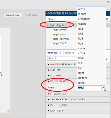
For apps made in AppDesigner, you can either set the pointer from the Design View or you can set the pointer property of the app’s UIFigure from the startup function using the second syntax shown above.

Part 2. How to change the pointer symbol dynamically

The pointer can be changed by setting specific conditions that trigger a change in the pointer symbol.

For example, the pointer can be temporarily changed to a busy-symbol when a button is pressed. This ButtonPushed callback function changes the pointer for 1 second.

function WaitasecondButtonPushed(app, event)
   % Change pointer for 1 second.
   set(app.UIFigure, 'Pointer','watch')
   pause(1)
   % Change back to default.
   set(app.UIFigure, 'Pointer','arrow')
   app.WaitasecondButton.Value = false;
end

The pointer can be changed every time it enters or leaves a uiaxes or any plotted object within the uiaxes. This is controlled by a set of pointer management functions that can be set in the app’s startup function.

iptSetPointerBehavior(obj,pointerBehavior) allows you to define what happens when the pointer enters, leaves, or moves within an object. Currently, only axes and axes objects seem to be supported for UIFigures.

iptPointerManager(hFigure,'enable') enables the figure’s pointer manager and updates it to recognize the newly added pointer behaviors.

The snippet below can be placed in the app’s startup function to change the pointer to crosshairs when the pointer enters the outerposition of a uiaxes and then change it back to the default arrow when it leaves the uiaxes.

% Define pointer behavior when pointer enter axes
pm.enterFcn = @(~,~) set(app.UIFigure, 'Pointer', 'crosshair');
pm.exitFcn  = @(~,~) set(app.UIFigure, 'Pointer', 'arrow');
pm.traverseFcn = [];
iptSetPointerBehavior(app.UIAxes, pm)

% Enable pointer manager for app
iptPointerManager(app.UIFigure,'enable'); 

Any function can be triggered when entering/exiting an axes object which makes the pointer management tools quite powerful. This snippet below defines a custom function cursorPositionFeedback() that responds to the pointer entering/exiting a patch object plotted within the uiaxes. When the pointer enters the patch, the patch color is changed to red, the pointer is changed to double arrows, and text appears in the app’s text area. When the pointer exits, the patch color changes back to blue, the pointer changes back to crosshairs, and the text area is cleared.

% Plot patch on uiaxes
hold(app.UIAxes, 'on')
region1 = patch(app.UIAxes,[1.5 3.5 3.5 1.5],[0 0 5 5],'b','FaceAlpha',0.07,...
    'LineWidth',2,'LineStyle','--','tag','region1');

% Define pointer behavior for patch
pm.enterFcn = @(~,~) cursorPositionFeedback(app, region1, 'in');
pm.exitFcn  = @(~,~) cursorPositionFeedback(app, region1, 'out');
pm.traverseFcn = [];
iptSetPointerBehavior(region1, pm)

% Enable pointer manager for app
iptPointerManager(app.UIFigure,'enable');

function cursorPositionFeedback(app, hobj, inout)
% When inout is 'in', change hobj facecolor to red and update textbox.
% When inout is 'out' change hobj facecolor to blue, and clear textbox.
% Check tag property of hobj to identify the object.
switch lower(inout)
    case 'in'
        facecolor = 'r';
        txt = 'Inside region 1';
        pointer = 'fleur';
    case 'out'
        facecolor = 'b';
        txt = '';
        pointer = 'crosshair';
end
hobj.FaceColor = facecolor;
app.TextArea.Value = txt;
set(app.UIFigure, 'Pointer', pointer)
end  

The app showing the demo below is attached.

Part 3. Create your own custom pointer symbol

1. Set the figure’s pointer property to ‘custom’.
2. Set the figure’s PointerShapeCData property to the custom pointer matrix. A custom pointer is defined by a 16x16 or 32x32 matrix where NaN values are transparent, 1=black, and 2=white.
3. Set the figure’s PointerShapeHotSpot to [m,n] where m and n are the coordinates that define the tip or "hotspot" of the matrix.

This demo uses the attached mat file to create a black hand pointer symbol.

iconData = load('blackHandPointer.mat');
uifig = uifigure(); 
uifig.Pointer = 'custom'; 
uifig.PointerShapeCData = iconData.blackHandIcon; 
uifig.PointerShapeHotSpot = iconData.hotspot;

Also see Jiro's pointereditor() function on the file exchange which allows you to draw your own pointer.

Today, I'm spotlighting Rik, our newest and the 31st MVP in MATLAB Answers. Two weeks ago, we just celebrated Ameer Hamza for reaching the MVP milestone. Today, we are thrilled that we have another new MVP!

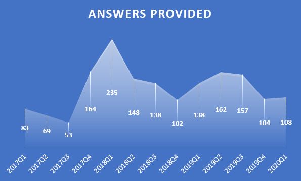
Since his first answer in Feb 2017, Rik has been contributing high-quality answers every quarter!

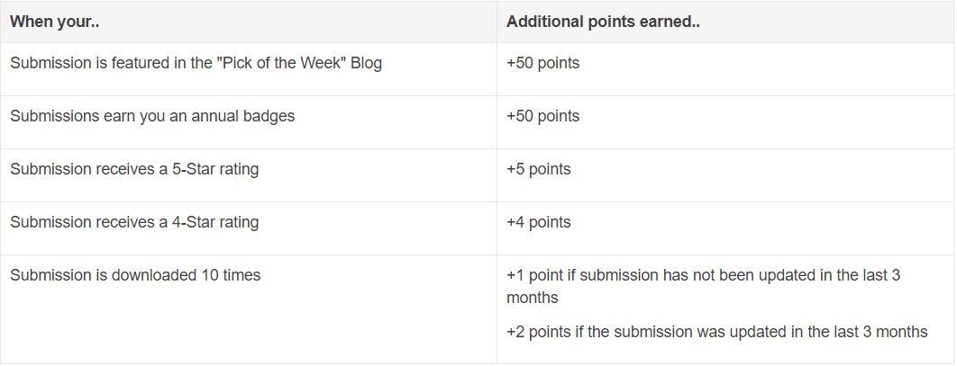
Besides those high-quality answers, Rik so far has submitted 21 files to File Exchange, one of which was chosen by MathWorks as the 'Pick of the Week'. Check the shining badge below.

Congratulations Rik! Thank you for your hard work and outstanding contributions.

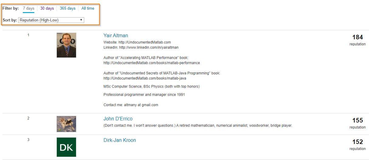
Today, I’m spotlighting Ameer Hamza , our newest MVP in Answers. Achieving MVP status is considered as a significant milestone and we know how hard it is to obtain 5,000 reputation points. Did you know Ameer earned 3000+ points and provided 1000+ answers in just 2 months? If you go to the leaderboard , you will find that Ameer ranks 1st in both 7-day leaderboard and 30-day leaderboard.

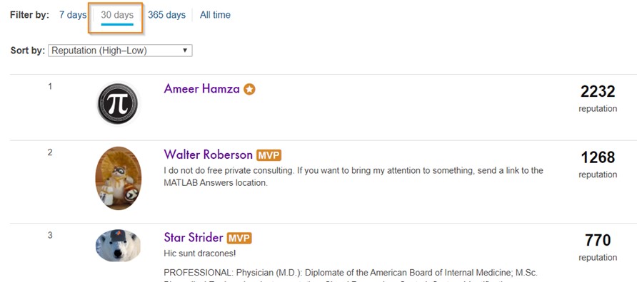
Due to Covid-19 pandemic, people have to stay at home and rely more on community for help. We have seen a significant increase in new questions per day. Luckily, we have a vibrant community! Many awesome contributors like Ameer double their effort to help people in need. Join me to thank Ameer and many other contributors!

Starting in r2020a, AppDesigner buttons and TreeNodes can display animated GIFs, SVG, and truecolor image arrays.

Every component in the App above is either a Button or a TreeNode!

Prior to r2020a the icon property of buttons and TreeNodes in AppDesigner supported JPEG, PNG, or GIF image files specified by a character vector or string array but did not support animation.

Here's how to display an animated GIF, SVG, or truecolor image in an App button or TreeNode starting in r2020a. And for the record, "GIF" is pronounced with a hard-g .

Display an animated GIF

Select the button or TreeNode from within AppDesigner > Design View and navigate to Component Browser > Inspector > Button dropdown list of properties (shown below). Select an animated GIF file and set the text and icon alignment properties.

To set the icon property programmatically,

app.Button.Icon = 'launch.gif';  % or "launch.gif"

The filename can be an image file on the Matlab path (see addpath ) or a full path to an image file.

Display SVG

Use “scalable vector graphics” files for high-resolution images that are scaled to different sizes while preserving their shape and retaining their clarity. A quick and easy way to remember which plotting function is assigned to each button in an app is to assign an image of the plot to the button.

After creating the figure, expand the axes by setting the position or outerposition property to [0 0 1 1] in normalized units and save the figure using File > Save as and select svg format. Save the image to the folder containing your app. Then follow the same procedure as animated GIFs.

Display truecolor image

A truecolor image comes in the form of an [m x n x 3] array where each m x n pixel color is specified by an RGB triplet (read more) . This feature allows you to dynamically create a digital image or to upload an image from a mat file rather than an image file.

In this example, a progress bar is created within the uibutton callback function and it’s updated within a loop. For a complete demo of this feature see this comment .

% Button pushed function: ProcessDataButton
function ProcessDataButtonPushed(app, event)
    % Change button name to "Processing"
    app.ProcessDataButton.Text = 'Processing...';
    % Put text on top of icon
    app.ProcessDataButton.IconAlignment = 'bottom';
    % Create waitbar with same color as button
    wbar = permute(repmat(app.ProcessDataButton.BackgroundColor,15,1,200),[1,3,2]);
    % Black frame around waitbar
    wbar([1,end],:,:) = 0;
    wbar(:,[1,end],:) = 0;
    % Load the empty waitbar to the button
    app.ProcessDataButton.Icon = wbar;
    % Loop through something and update waitbar
    n = 10;
    for i = 1:n
        % Update image data (royalblue)
        % if mod(i,10)==0 % update every 10 cycles; improves efficiency
         currentProg = min(round((size(wbar,2)-2)*(i/n)),size(wbar,2)-2);
         RGB = app.ProcessDataButton.Icon;
         RGB(2:end-1, 2:currentProg+1, 1) = 0.25391; % (royalblue)
         RGB(2:end-1, 2:currentProg+1, 2) = 0.41016;
         RGB(2:end-1, 2:currentProg+1, 3) = 0.87891;

           app.ProcessDataButton.Icon = RGB;
          % Pause to slow down animation
          pause(.3)
          % end
      end
      % remove waitbar
      app.ProcessDataButton.Icon = '';
      % Change button name
      app.ProcessDataButton.Text = 'Process Data';
  end

The for-loop above was improved on Feb-11-2022.

Credit for the black & teal GIF icons: lordicon.com

The File Exchange team is excited to announce that File Exchange now supports GitHub Releases!

Contributors can now develop software projects in GitHub without having to manually sync and maintain the same code in File Exchange.

To start using this feature, choose 'GitHub Releases' option when you update your existing File Exchange submission or link a new repository to File Exchange.

When you link your GitHub repository to File Exchange using GitHub Releases, your File Exchange submission will automatically update when you create a new release in GitHub that is compatible with File Exchange. In addition, if you package your code as a toolbox (.mltbx) and attach the toolbox package to your latest GitHub release, File Exchange will provide the toolbox to your users for download. If you do not attach a toolbox to the release, File Exchange will provide the zip release asset for download.

See this page for more details.

We encourage you to try out this feature and let us know of any feedback you have by replying below.

This week is National Volunteer Week in the USA and Canada and to celebrate, I’d like to pay tribute to the volunteers in the Matlab Central Answers forum who have given countless hours to help total strangers make progress in their education, careers, and hobbies.

As of April 20, 2020, there have been 375,869 [1,2] questions asked by 183,968 [3] contributors dating back to the earliest existing question on January 4, 2011.

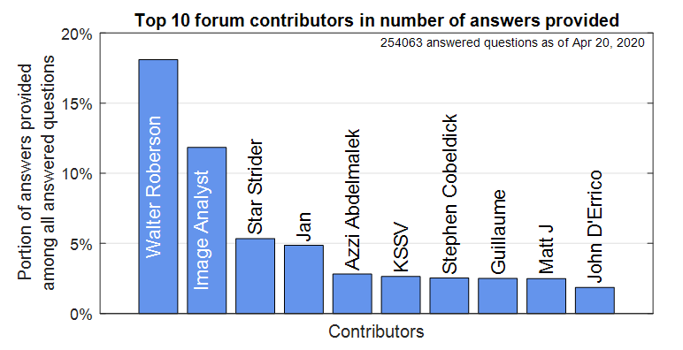
41,890 volunteers have contributed at least one answer leading up to 68% of the questions answered.

There is no contribution too small for earning well-deserved recognition and appreciation. A single answer or comment may benefit countless individuals who finally find the ideal solution to a problem that kept them up at night.

A number of volunteers in the forum have contributed far and beyond the imaginable and have shared so much of their time and expertise that it’s difficult to fathom. The bar graph below shows the top 10 volunteers in the forum by the number of answers provided. It’s hard to believe that Walter Roberson , a single individual ( we think ), has contributed a portion of answers equal to more than 18% of answered questions in the forum [4]. The top two volunteers, adding Image Analyst , contributed enough answers to equal almost 30% of the answered questions. These folks along with many others not listed in the bar graph who can be found on the contributors page are the foundation of so many Matlab users’ success including my own from June 2014, when I asked my first question.

Whether you’ve come to the forum to look for an answer or to write an answer, you’re undoubtedly standing on the shoulders of giants.

Footnotes

1. Based on the number of answered and unanswered questions listed in the ‘Status’ table in recently added questions .
2. Questions and answers posted by the MathWorks Support Team are not included in the data presented here, though much appreciated.
3. The number of people who provided an answer is based on sorting the contributors page by ‘answers given’ in descending order.
4. Since a contributor can write more than one answer to a question, we can’t easily measure the number of questions answered by a contributor.

New to r2020a, leapseconds() creates a table showing all leap seconds recognized by the datetime data type.

>> leapseconds()
ans =
  27×2 timetable
       Date        Type    CumulativeAdjustment
    ___________    ____    ____________________
    30-Jun-1972     +              1 sec       
    31-Dec-1972     +              2 sec       
    31-Dec-1973     +              3 sec       
    31-Dec-1974     +              4 sec       
    31-Dec-1975     +              5 sec       
             << 21 rows removed >>
    31-Dec-2016     +             27 sec   

Leap seconds can covertly sneak into your data and cause errors that are difficult to resolve if the leap seconds go undetected. A leap second was responsible for crashing Reddit , Mozilla, Yelp, LinkedIn and other sites in 2012.

Detect leap seconds present in a vector of years

% Define a vector of years
t = 2005:2008; 

allLeapSeconds = leapseconds(); 
isYearWithLeapSecond = ismember(t,year(allLeapSeconds.Date));

% Show years that contain a leap second
t(isYearWithLeapSecond)
ans =
        2005        2008

Detect leap seconds present in a vector of months

% Define a vector of months 
t = datetime(1972, 1, 1) + calmonths(0:11);

t.Format = 'MMM-yyyy';
allLeapSeconds = leapseconds(); 
[tY,tM] = ymd(t); 
[leapSecY, leapSecM] = ymd(allLeapSeconds.Date); 
isMonthWithLeapSecond = ismember([tY(:),tM(:)], [leapSecY, leapSecM], 'rows');

% Show months that contain a leap second
t(isMonthWithLeapSecond)
ans = 
  1×2 datetime array
   Jun-1972   Dec-1972

List all leap seconds in your lifetime

% Enter your birthday in mm/dd/yyyy hh:mm:ss format
yourBirthday = '01/15/1988 14:30:00'; 

yourTimeRange = timerange(datetime(yourBirthday), datetime('now')); 
allLeapSeconds = leapseconds(); 
lifeLeapSeconds = allLeapSeconds(yourTimeRange,:);
lifeLeapSeconds.YourAge = lifeLeapSeconds.Date - datetime(yourBirthday);
lifeLeapSeconds.YourAge.Format = 'y';

% Show table
fprintf('\n Leap seconds in your lifetime:\n')
disp(lifeLeapSeconds)

Leap seconds in your lifetime:
       Date        Type    CumulativeAdjustment     YourAge  
    ___________    ____    ____________________    __________
    31-Dec-1989     +             15 sec           1.9587 yrs
    31-Dec-1990     +             16 sec            2.958 yrs
                        << 8 rows removed >>
    30-Jun-2012     +             25 sec           24.456 yrs
    30-Jun-2015     +             26 sec           27.454 yrs
    31-Dec-2016     +             27 sec            28.96 yrs

What is a leap second?

A second is defined as the time it takes a cesium-133 atom to oscillate 9,192,631,770 times under controlled conditions. The transition frequency is so precise that it takes 100 million years to gain 1 second of error [1]. If the earth’s rotation were perfectly synchronized to the atomic second, a day would be 86,400 seconds. But the earth’s rate of rotation is affected by climate, winds, atmospheric pressure, and the rate of rotation is gradually decreasing due to tidal friction [2,3]. Several months before the expected difference between the atomic clock-based time (UTC) and universal time (UT1) reaches +/- 0.9 seconds the IERS authorizes the addition (or subtraction) of 1 leap second (see plot below). Since the first leap second in 1972, all leap second adjustments have been made on the last day of June or December and all adjustments have been +1 second which explains the + signs in the type column of the leapseconds() table.

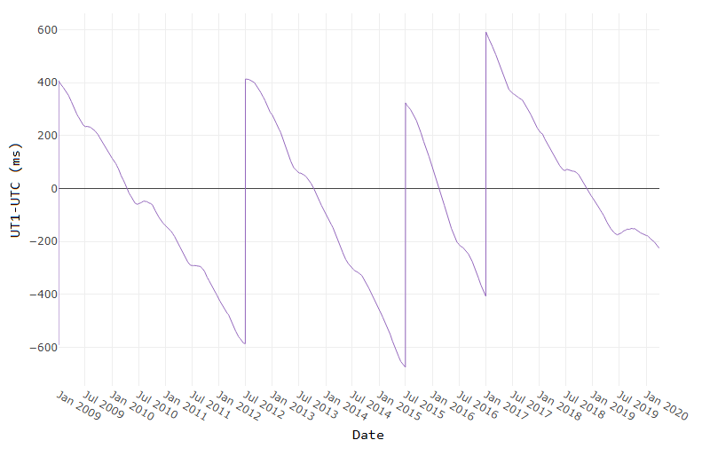
[ Image source ]

How to reference the leap second schedule in your code

Since leap second adjustments are not regularly timed, you can record the official IERS Bulletin C version used at the time of your analysis by accessing the 2nd output to leapseconds().

[T,vers] = leapseconds

What do leap seconds look like in datetime values?

A minute typically has 60 seconds spanning from 0:59. A minute containing a leap second has 61 seconds spanning from 0:60.

December 30, 2016 was a normal day. If we add the usual 86400 seconds to the start of that day, the result is the start of the next day.

d = datetime(2016, 12, 30, 'TimeZone','UTCLeapSeconds') + seconds(86400)
d = 
  datetime
   2016-12-31T00:00:00.000Z

The next day, December 31, 2016, had a leap second. If we add 86400 seconds to the start of that day, the result is not the start of the next day.

d = datetime(2016, 12, 31, 'TimeZone','UTCLeapSeconds') + seconds(86400)
d = 
  datetime
   2016-12-31T23:59:60.000Z

When will the next leap second be?

As of the current date (April 2020) the timing of the next leap second is unknown. Based on the data from the plot above, what's your guess?

References

1. https://www.timeanddate.com/time/how-do-atomic-clocks-work.html
2. https://www.nasa.gov/centers/goddard/news/topstory/2003/0210rotation.html
3. https://en.wikipedia.org/wiki/%CE%94T#Universal_time