主要内容
搜索
In the past two years, large language models have brought us significant changes, leading to the emergence of programming tools such as GitHub Copilot, Tabnine, Kite, CodeGPT, Replit, Cursor, and many others. Most of these tools support code writing by providing auto-completion, prompts, and suggestions, and they can be easily integrated with various IDEs.
As far as I know, aside from the MATLAB-VSCode/MatGPT plugin, MATLAB lacks such AI assistant plugins for its native MATLAB-Desktop, although it can leverage other third-party plugins for intelligent programming assistance. There is hope for a native tool of this kind to be built-in.
We are thrilled to see the incredible short movies created during Week 3. The bar has been set exceptionally high! This week, we invited our Community Advisory Board (CAB) members to select winners. Here are their picks:
Mini Hack Winners - Week 3
Game:
Holidays:
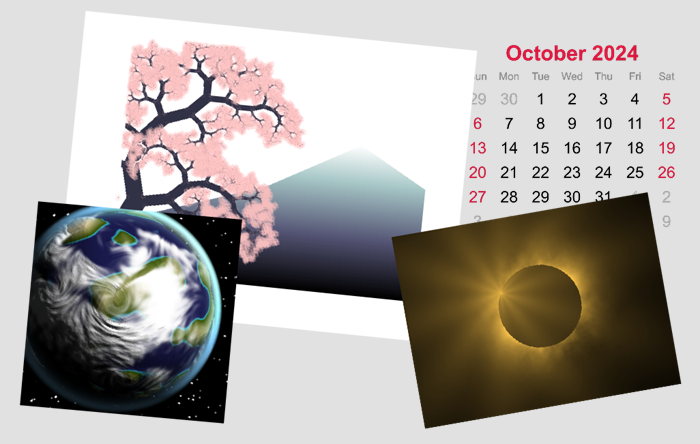
Fractals:
Realism:
Great Remixes:
Seamless loop:
Fun:
Weekly Special Prizes
Thank you for sharing your tips & tricks with the community. You won a limited-edition MATLAB Shorts.
We still have plenty of MATLAB Shorts available, so be sure to create your posts before the contest ends. Don't miss out on the opportunity to showcase your creativity!
Just in two weeks, we already have 150+ entries! We are so impressed by your creative styles, artistic talents, and ingenious programming techniques.
Now, it’s time to announce the weekly winners!
Mini Hack Winners - Week 2
Seamless loop:
Nature & Animals:
Game:
Synchrony:
Remix of previous Mini Hack entries
Movie:
Congratulations to all winners! Each of you won your choice of a T-shirt, a hat, or a coffee mug. We will contact you after the contest ends.
In week 3, we’d love to see and award entries in the ‘holiday’ category.
Weekly Special Prizes
Thank you for sharing your tips & tricks with the community. You won limited-edition MATLAB Shorts.
We highly encourage everyone to share various types of content, such as tips and tricks for creating animations, background stories of your entry, or learnings you've gained from the contest.
There are so many incredible entries created in week 1. Now, it’s time to announce the weekly winners in various categories!
Nature & Space:
Seamless Loop:
Abstract:
Remix of previous Mini Hack entries:
Early Discovery
Holiday:
Congratulations to all winners! Each of you won your choice of a T-shirt, a hat, or a coffee mug. We will contact you after the contest ends.
In week 2, we’d love to see and award more entries in the ‘Seamless Loop’ category. We can't wait to see your creativity shine!
Tips for Week 2:
1.Use AI for assistance
The code from the Mini Hack entries can be challenging, even for experienced MATLAB users. Utilize AI tools for MATLAB to help you understand the code and modify the code. Here is an example of a remix assisted by AI. @Hans Scharler used MATLAB GPT to get an explanation of the code and then prompted it to ‘change the background to a starry night with the moon.’
2. Share your thoughts
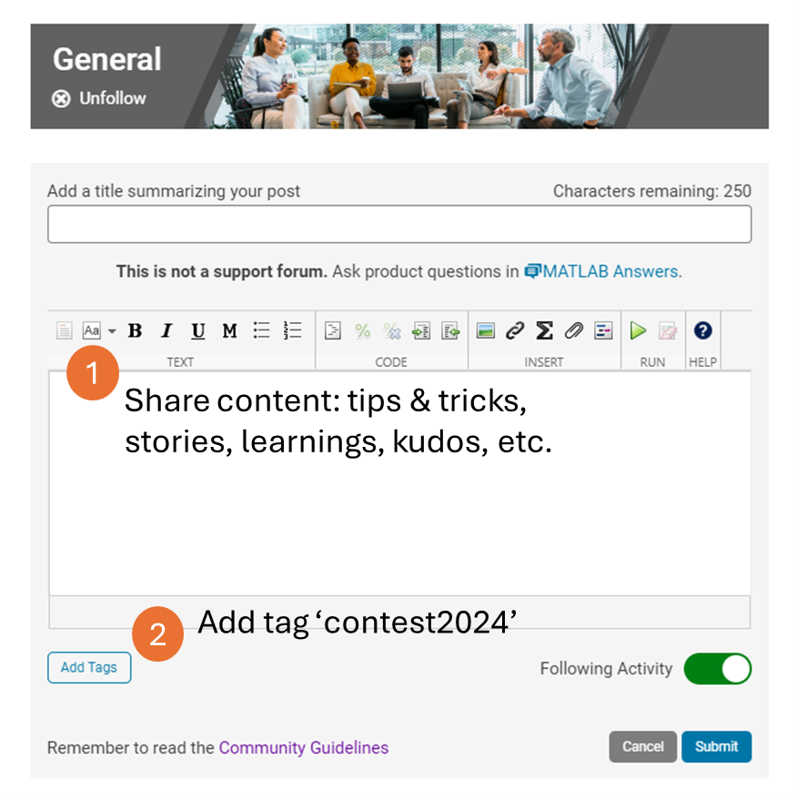
Share your tips & tricks, experience of using AI, or learnings with the community. Post your knowledge in the Discussions' general channel (be sure to add the tag 'contest2024') to earn opportunities to win the coveted MATLAB Shorts.
3. Ensure Thumbnails Are Displayed:
You might have noticed that some entries on the leaderboard lack a thumbnail image. To fix this, ensure you include ‘drawframe(1)’ in your code.
Over the past week, we have seen many creative and compelling short movies! Now, let the voting begin! Cast your votes for the short movies you love. Authors, share your creations with friends, classmates, and colleagues. Let's showcase the beauty of mathematics to the world!
We know that one of the key goals for joining the Mini Hack contest is to LEARN! To celebrate knowledge sharing, we have special prizes—limited-edition MATLAB Shorts—up for grabs!
These exclusive prizes can only be earned through the MATLAB Shorts Mini Hack contest. Interested? Share your knowledge in the Discussions' general channel (be sure to add the tag 'contest2024') to earn opportunities to win the coveted MATLAB Shorts. You can share various types of content, such as tips and tricks for creating animations, background stories of your entry, or learnings you've gained from the contest. We will select different types of winners each week.
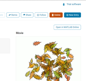
We also have an exciting feature announcement: you can now experiment with code in MATLAB Online. Simply click the 'Open in MATLAB Online' button above the movie preview section. Even better! ‘Open in MATLAB Online’ is also available in previous Mini Hack contests!
We look forward to seeing more amazing short movies in Week 2!
We're excited to announce that the 2024 Community Contest—MATLAB Shorts Mini Hack starts today! The contest will run for 5 weeks, from Oct. 7th to Nov. 10th.
What creative short movies will you create? Let the party begin, and we look forward to seeing you all in the contest!
If I go to a paint store, I can get foldout color charts/swatches for every brand of paint. I can make a selection and it will tell me the exact proportions of each of base color to add to a can of white paint. There doesn't seem to be any equivalent in MATLAB. The common word "swatch" doesn't even exist in the documentation. (?) One thinks pcolor() would be the way to go about this, but pcolor documentation is the most abstruse in all of the documentation. Thanks 1e+06 !
As pointed out in Doxygen comments in code generated with Simulink Embedded Coder - MATLAB Answers - MATLAB Central (mathworks.com), it would be nice that Embedded Coder has an option to generate Doxygen-style comments for signals of buses, i.e.:
/** @brief <Signal desciption here> **/
This would allow static analysis tools to parse the comments. Please add that feature!
Dear contest participants,
The 2024 Community Contest—MATLAB Shorts Mini Hack—is just one week away! Last year, we challenged you to create a 48-frame, 2-second animation. This year, we're doubling the fun by increasing the frame count to 96 and adding audio support. Your mission? Create a short movie!
As always, whether you are a seasoned MATLAB user or just a beginner, you can participate in the contest and have opportunities to win amazing prizes.
Timeframe:
- The contest will run for 5 weeks, from Oct. 7th to Nov. 10th, Eastern Time.
General Rules:
- The first week is dedicated to entry creation, and the fifth week is reserved for voting only.
- Create a 96-frame, 4-second animation and add audio. We will loop it 3 times to create a 12-second short movie for you.
- The character limit remains at 2,000 characters.
Prizes
- You will have opportunities to win compelling prizes, including Amazon gift cards, MathWorks T-shirts, and virtual badges. We will give out both weekly prizes and grand prizes.
Warm-up!
With one week left before the contest begins, we recommend you warm up by reading a fantastic article: Walkthrough: making Little Nemo's airship in MATLAB by @Tim. The article shares both technical insights and the challenges encountered along the way.
The MATLAB Central Community Team
Dear MATLAB contest enthusiasts,
In the 2023 MATLAB Mini Hack Contest, Tim Marston captivated everyone with his incredible animations, showcasing both creativity and skill, ultimately earning him the 1st prize.
We had the pleasure of interviewing Tim to delve into his inspiring story. You can read the full interview on MathWorks Blogs: Community Q&A – Tim Marston.
Last question: Are you ready for this year’s Mini Hack contest?
As far as I know, starting from MATLAB R2024b, the documentation is defaulted to be accessed online. However, the problem is that every time I open the official online documentation through my browser, it defaults or forcibly redirects to the documentation hosted site for my current geographic location, often with multiple pop-up reminders, which is very annoying!
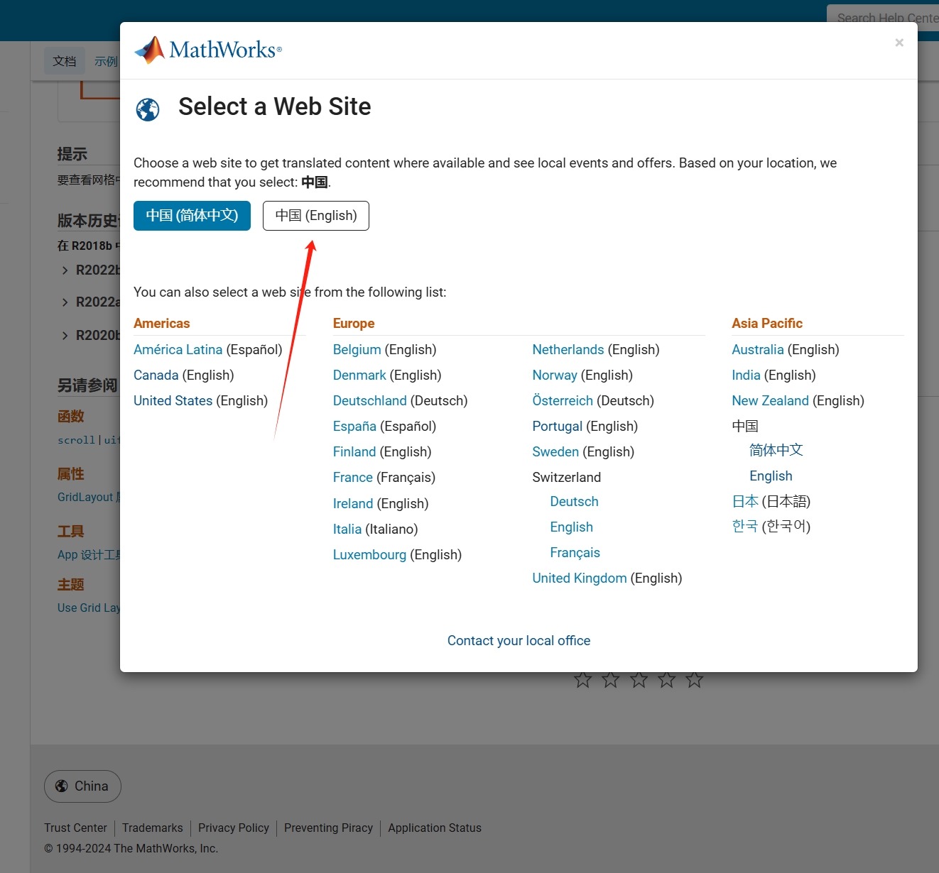
Suggestion: Could there be an option to set preferences linked to my personal account so that the documentation defaults to my chosen language preference without having to deal with “forced reminders” or “forced redirection” based on my geographic location? I prefer reading the English documentation, but the website automatically redirects me to the Chinese documentation due to my geolocation, which is quite frustrating!
----------------2024.12.13 update-----------------
Although the above issue was resolved by technical support, subsequent redirects are still causing severe delays...
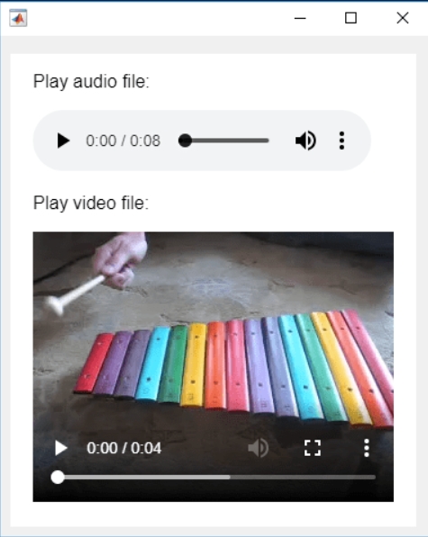
In the past two years, MATHWORKS has updated the image viewer and audio viewer, giving them a more modern interface with features like play, pause, fast forward, and some interactive tools that are more commonly found in typical third-party players. However, the video player has not seen any updates. For instance, the Video Viewer or vision.VideoPlayer could benefit from a more modern player interface. Perhaps I haven't found a suitable built-in player yet. It would be great if there were support for custom image processing and audio processing algorithms that could be played in a more modern interface in real time.
Additionally, I found it quite challenging to develop a modern video player from scratch in App Designer.(If there's a video component for that that would be great)
-----------------------------------------------------------------------------------------------------------------
BTW,the following picture shows the built-in function uihtml function showing a more modern playback interface with controls for play, pause and so on. But can not add real-time image processing algorithms within it.
I was browsing the MathWorks website and decided to check the Cody leaderboard. To my surprise, William has now solved 5,000 problems. At the moment, there are 5,227 problems on Cody, so William has solved over 95%. The next competitor is over 500 problems behind. His score is also clearly the highest, approaching 60,000.
I've been working on some matrix problems recently(Problem 55225)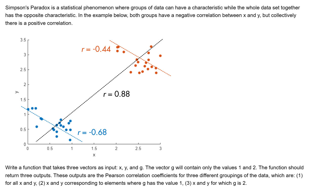
and this is my code
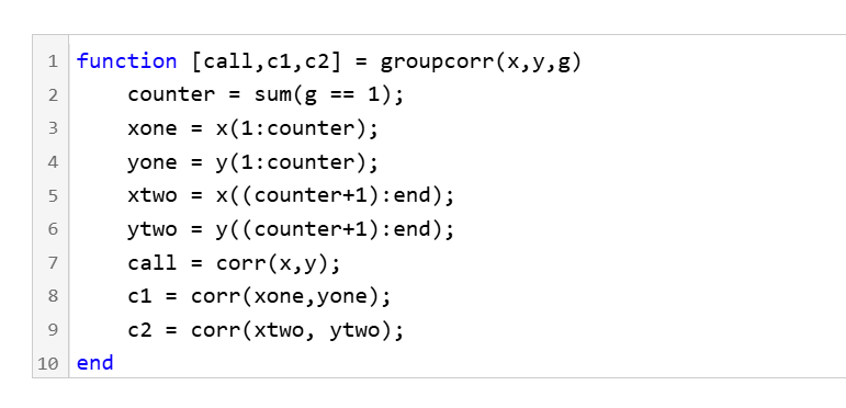
It turns out that "Undefined function 'corr' for input arguments of type 'double'." However, should't the input argument of "corr" be column vectors with single/double values? What's even going on there?
isequaln exists to return true when NaN==NaN.
unique treats NaN==NaN as false (as it should) requiring NaN to be replaced if NaN is not considered unique in a particular application. In my application, I am checking uniqueness of table rows using [table_unique,index_unique]=unique(table,"rows","sorted") and would prefer to keep NaN as NaN or missing in table_unique without the overhead of replacing it with a dummy value then replacing it again. Dummy values also have the risk of matching existing values in the table, requiring first finding a dummy value that is not in the table.
uniquen (similar to isequaln) would be more eloquent.
Please point out if I am missing something!
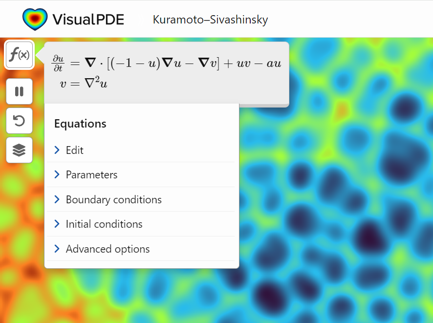
A library of runnable PDEs. See the equations! Modify the parameters! Visualize the resulting system in your browser! Convenient, fast, and instructive.
Hi everyone,
I've recently joined a forest protection team in Greece, where we use drones for various tasks. This has sparked my interest in drone programming, and I'd like to learn more about it. Can anyone recommend any beginner-friendly courses or programs that teach drone programming?
I'm particularly interested in courses that focus on practical applications and might align with the work we do in forest protection. Any suggestions or guidance would be greatly appreciated!
Thank you!
"What are your favorite features or functionalities in MATLAB, and how have they positively impacted your projects or research? Any tips or tricks to share?
function ans = your_fcn_name(n)
n;
j=sum(1:n);
a=zeros(1,j);
for i=1:n
a(1,((sum(1:(i-1))+1)):(sum(1:(i-1))+i))=i.*ones(1,i);
end
disp
I am trying to earn my Intro to MATLAB badge in Cody, but I cannot click the Roll the Dice! problem. It simply is not letting me click it, therefore I cannot earn my badge. Does anyone know who I should contact or what to do?
您也可以从以下列表中选择网站:
美洲
- América Latina (Español)
- Canada (English)
- United States (English)
欧洲
- Belgium (English)
- Denmark (English)
- Deutschland (Deutsch)
- España (Español)
- Finland (English)
- France (Français)
- Ireland (English)
- Italia (Italiano)
- Luxembourg (English)
- Netherlands (English)
- Norway (English)
- Österreich (Deutsch)
- Portugal (English)
- Sweden (English)
- Switzerland
- United Kingdom(English)
亚太
- Australia (English)
- India (English)
- New Zealand (English)
- 中国
- 日本Japanese (日本語)
- 한국Korean (한국어)