搜索
So, I'm trying to find the rate of climb against the velocity.
Both of these variables are 1 x 100 vectors.
rate of climb = v.*(T-D)./w
where w is a constant. t,d and v are all arrays of 1 x 100 row vectors. I was wondering ways to find the derivative at the local maximum. Examples would be appreciated.
I'm using app designer to link it with one simulink model of mine. I had used editfield (numeric) in app such that inputs to simulink model can be given through this app. The variables declared in app code will be used in simulink model. But when I give numeric inputs to app and run, the variables in simulink are showing it as 0 in the base workspace too.
Syntax used for assigning a variable to editfield is:
assignin("base", "variablename", app.EditFieldName.Value);
Please give me the solution to this.
This is my code
%send food and medicine in flood situation
% 1. create map
clc
clear
tic
map3D = occupancyMap3D; % create space for
[xGround,yGround,zGround] = meshgrid(0:240,0:350, 0); %set floor x=500 y=500
xyzGround = [xGround(:) yGround(:) zGround(:)]; %use for mergegrid
occval = 0;
setOccupancy(map3D,xyzGround,occval)
% xspace = 20 y = 45 create
[xB1, yB1, zB1] = meshgrid(50:130, 60:110, 0:20); %unionmall
[xB2, yB2, zB2] = meshgrid(80:250, 160:240, 0:30); %centralladprao
[xB3, yB3, zB3] = meshgrid(220:250, 290:340, 0:60); %centarahotel
[xB4, yB4, zB4] = meshgrid(0:30, 10:40, 0:80); %condo
[xB5, yB5, zB5] = meshgrid(150:170, 80:100, 0:10); %house1
[xB6, yB6, zB6] = meshgrid(180:200, 80:100, 0:10); %house2
[xB7, yB7, zB7] = meshgrid(210:230, 80:100, 0:10); %house3
[xB11, yB11, zB11] = meshgrid(240:270, 80:100, 0:10); %house7
[xB8, yB8, zB8] = meshgrid(150:170, 50:70, 0:10); %house4
[xB9, yB9, zB9] = meshgrid(180:200, 50:70, 0:10); %house5
[xB10, yB10, zB10] = meshgrid(210:230, 50:70, 0:10); %house6
[xB12, yB12, zB12] = meshgrid(240:270, 50:70, 0:10); %house8
[xB13, yB13, zB13] = meshgrid(200:260, 0:30, 0:13); %villageoffice
xyzB = [xB1(:), yB1(:), zB1(:);
xB2(:), yB2(:), zB2(:);
xB3(:), yB3(:), zB3(:);
xB4(:), yB4(:), zB4(:);
xB5(:), yB5(:), zB5(:);
xB6(:), yB6(:), zB6(:);
xB7(:), yB7(:), zB7(:);
xB8(:), yB8(:), zB8(:);
xB9(:), yB9(:), zB9(:);
xB10(:), yB10(:), zB10(:);
xB11(:), yB11(:), zB11(:);
xB12(:), yB12(:), zB12(:);
xB13(:), yB13(:), zB13(:);];
obs = 0.65; % ;=not show in command window
my3Dmap = map3D;
updateOccupancy(my3Dmap,xyzB,obs);
%show(my3Dmap);
% 2. distination
%my3Dmap.FreeThreshold = my3Dmap.OccupiedThreshold;
startPose = [50 60 25 pi/2;
250 310 65 pi/2;
100 170 35 pi/2;
100 30 85 pi/2;
155 90 15 pi/2;
250 60 15 pi/2;
160 60 15 pi/2
220 15 20 pi/2;];
goalPose = startPose;
ss = ExampleHelperUAVStateSpace("MaxRollAngle",pi/3,...
"AirSpeed",5,...
"FlightPathAngleLimit",[-0.5 0.5],...
"Bounds",[-10 400;-10 4000; -10 100; -pi pi]);
%threshold = [(goalPose-0.5)' (goalPose+0.5)'; -pi pi];
%setWorkspaceGoalRegion(ss,goalPose,threshold)
sv = validatorOccupancyMap3D(ss,"Map",my3Dmap);
sv.ValidationDistance = 0.5;
planner = plannerBiRRT(ss,sv);
planner.MaxConnectionDistance = 100;
%planner.GoalBias = 0.10;
%1,0.1,0.15,0.5,0.2,0.13,
planner.MaxIterations = 100000;
%planner.GoalReachedFcn = @(~,x,y)(norm(x(1:3)-y(1:3)) < 5);
planner.MaxNumTreeNodes = 10000;
numPose = length(startPose);
distances = zeros(numPose, numPose);
for i = 1:numPose
for j = 1:numPose
if i ~= j
rng(100, "twister");
start = [startPose(i,1), startPose(i,2), startPose(i,3), startPose(i,4)];
goal = [goalPose(j,1), goalPose(j,2), goalPose(j,3), goalPose(j,4)];
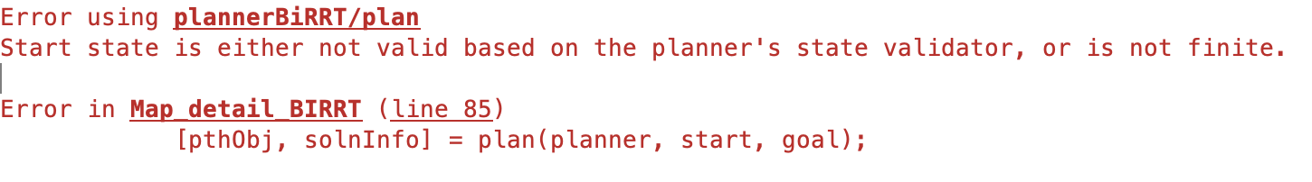
[pthObj, solnInfo] = plan(planner, start, goal);
smoothWaypointsObj = exampleHelperUAVPathSmoothing(ss, sv, pthObj);
distances(i, j) = pathLength(smoothWaypointsObj);
end
end
end
toc
and the error below
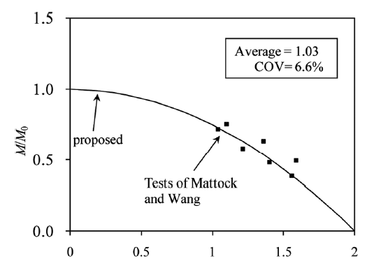 Hi, I have this equation for moment-axial force interaction: 0.25*(M/M0)^2 + (N/N0) = 1. This equation produces the following curve. Now, I need to make a change to this equation so that the first term becomes (M/M0)^2, and the second term can be changed while keeping (N/N0). The other side of the equation remains the same. ((M/M0)^2+?? = 1). I need to get the same curve as in the figure.
Hello everyone,
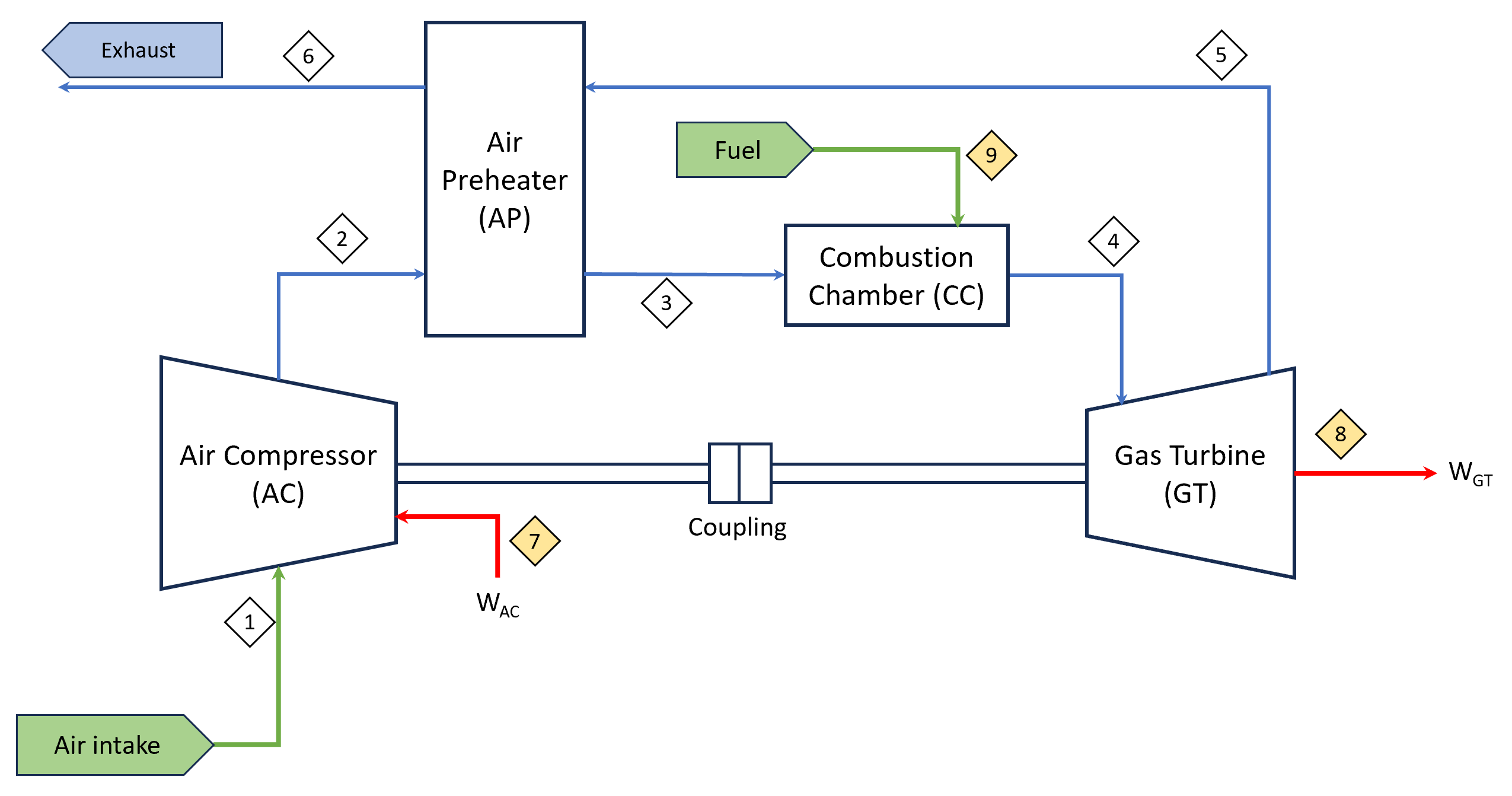
I am trying simulate a gas turbine system for my course on modelling and optimization of energy system. I have come out with a design consisting of a compressor, air preheater, combustion chamber and gas turbine. When I try to do the modelling in Simulink, I couldnt find something similar to combustion chamber. Does anyone have any experience in doing this?
Orginal Design:
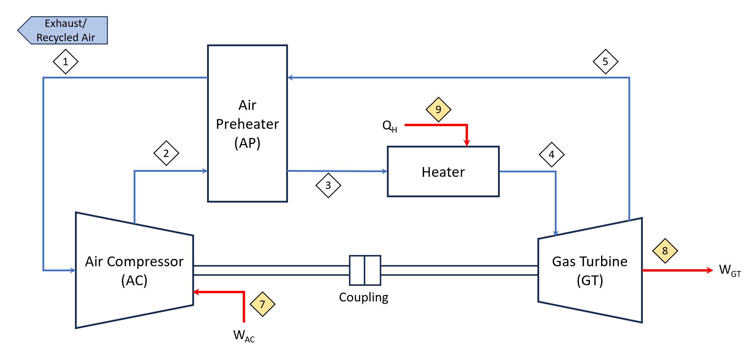
I have also amended it and come out with second design, where I change to combustion chamber to a heater and the exhaust air is recycled back to air compressor, making it a closed loop system. But I am also unable to find heater from the simulink library, the closest i can get is convective heat transfer. Can someone help on this too and if the closed loop system is feasible to model?
Design 2 :
Hi everyone,
for my thesis project I would need to get, every second of the simulation, real-time output data from a Simulink model, without using Simulink Real-Time, as it supports only Speedgoat Hardware. Is there a particular set of blocks for that purpose?
I have to provide that real-time data to hardware for an Hardware in the Loop Simulation so I will need to be able also to receive, as an input, data from the hardware to the Simulink model, again every second of the simulation, to close the loop of the simulation.
Thank you in advance for your support.
Hi! I am using matlab inbuilt plot option( without typing code) to plot the data. This joins the data points using straight line by default. What will be the easiest way to plot if I want curve to join the points instead?
Quick answer: Add set(hS,'Color',[0 0.4470 0.7410]) to code line 329 (R2023b).
Explanation: Function corrplot uses functions plotmatrix and lsline. In lsline get(hh(k),'Color') is called in for cycle for each line and scatter object in axes. Inside the corrplot it is also called for all axes, which is slow. However, when you first set the color to any given value, internal optimization makes it much faster. I chose [0 0.4470 0.7410], because it is a default color for plotmatrix and corrplot and this setting doesn't change a behavior of corrplot.
Suggestion for a better solution: Add the line of code set(hS,'Color',[0 0.4470 0.7410]) to the function plotmatrix. This will make not only corrplot faster, but also any other possible combinations of plotmatrix and get functions called like this:
h = plotmatrix(A);
% set(h,'Color',[0 0.4470 0.7410])
for k = 1:length(h(:))
get(h(k),'Color');
end
I keep getting this error message when trying to run my code, I'm confident my wiring is correct and I do not know what this error means-
Library 'Servo' is not uploaded to the board. Clear the current Arduino object and recreate it to include the appropriate library. For a list of available libraries, type 'listArduinoLibraries'.
here is my code
a=arduino();
s1 = servo(a, 'D9', 'MinPulseDuration', 700*10^-6, 'MaxPulseDuration', 2300*10^-6);
writePosition(s1,0);
userResponse = "yes";
while userResponse == "yes"
chicken = input("Insert your resistor");
voltage = readVoltage(a, "A0");
if voltage < 1.67155
resistor = "47k";
writePosition(s1,0.25);
minR = 47000 * 0.95;
maxR = 47000 * 1.05;
elseif voltage < 3.53128
resistor = "10k";
writePosition(s1,0.5);
minR = 10000 * 0.95;
maxR = 10000 * 1.05;
elseif voltage < 4.69941
resistor = "1k";
writePosition(s1,0.75);
minR = 1000 * 0.95;
maxR = 1000 * 1.05;
else
resistor = "330";
writePosition(s1,1);
minR = 330 * 0.95;
maxR = 330 * 1.05;
end
resistance = voltageToResistance(voltage);
withinTolerance = (resistance >= minR && resistance <= maxR);
disp(resistor)
if withinTolerance == 1
writeDigitalPin(a, "D4", 1);
writeDigitalPin(a, "D5", 0);
%disp("green")
else
writeDigitalPin(a, "D4", 0);
writeDigitalPin(a, "D5", 1);
%disp("Red")
end
userResponse = input("Would you like to check another resistor? ","s");
writePosition(s1,0);
writeDigitalPin(a, "D4", 0);
writeDigitalPin(a, "D5", 0);
end
How to Simulate a Synchronous Compensator in Simulink?
We are thrilled to announce the grand prize winners of our MATLAB Flipbook contest! This year, we invited the MATLAB Graphics Infrastructure team, renowned for their expertise in exporting and animation workflows, to be our judges. After careful consideration, they have selected the top three winners:
Judge comments: Creative and realistic rendering with well-written code
2nd place - Christmas Tree / Zhaoxu Liu
Judge comments: Festive and advanced animation that is appropriate to the current holiday season.
Judge comments: Nice translation of existing shader logic to MATLAB that produces an advanced and appealing visual effect.
In addition, after validating the votes, we are pleased to announce the top 10 participants on the leaderboard:
- Tim
- Zhaoxu Liu / slandarer
- KARUPPASAMYPANDIYAN M
- Dhimas Mahardika S.Si., M.Mat
- Augusto Mazzei
- Jenny Bosten
- Lucas
- Jr
- Victoria
- ME
Congratulations to all! Your creativity and skills have inspired many of us to explore and learn new skills, and make this contest a big success!
The MATLAB Flipbook Mini Hack contest has concluded! During the 4 weeks, over 600 creative animations have been created. We had a lot of fun and a great learning experience! Thank you, everyone!
Now it’s the time to announce week 4 winners. Note that grand prize winners will be announced shortly after we validate votes on winning entries.
Realism:
Holiday & Season:
Abstract:
Cartoon:
Congratulations, weekly winners!We will reach out to you shortly for your prizes.
The MATLAB AI Chat Playground is now open to the whole community! Answer questions, write first draft MATLAB code, and generate examples of common functions with natural language.
The playground features a chat panel next to a lightweight MATLAB code editor. Use the chat panel to enter natural language prompts to return explanations and code. You can keep chatting with the AI to refine the results or make changes to the output.

Give it a try, provide feedback on the output, and check back often as we make improvements to the model and overall experience.
Looking for an opportunity to practice your AI skills on a real-world problem? Interested in AI for climage change? Sign up for the Kelp Wanted challenge, which tasks participants with developing an algorithm that can detect the presence of kelp forests from satellite images.
Participants of all skill levels from anywhere in the world are welcome to compete!
MathWorks provides the following resources for all participants:
Hello,
I have to draw root-locus for longitudinal motion; Short Period Mode and Phugoid Mode. Here is a code
%% Dynamics
Vp = 111.174
A_lon = [-0.0283 0.3139 -11.0665 -32.0344;
-0.4204 -1.5452 108.6931 -3.2616;
0.0205 -0.2011 -3.5080 0;
0 0 1 0]
B_lon = [0.0115 0.1150;
-0.2185 0;
-0.3591 0;
0 0]
C_lon = [1 0 0 0;
0 -1 0 Vp]
%% LQR Servo Design
A_servo = [A_lon zeros(4,2);
-C_lon zeros(2,2)]
B_servo = [B_lon ; zeros(2,2)]
n = 100; a = logspace(-2,2,n);
for i = 1:n
Q = a(i)*[1 0 0 0 0 0;
0 1 0 -Vp 0 0;
0 0 0 0 0 0;
0 -Vp 0 power(Vp,2) 0 0;
0 0 0 0 1 0;
0 0 0 0 0 1];
R = eye(2);
[K,S,P] = lqr(A_servo,B_servo,Q,R);
p_cl = P;
cl_sh(i,1) = p_cl(5); cl_sh(i,2) = p_cl(6);
cl_ph(i,1) = p_cl(3); cl_ph(i,2) = p_cl(4);
end
%% Plot
figure;
plot(real(cl_sh(:,1)), imag(cl_sh(:,1)), '+', real(cl_sh(:,2)), imag(cl_sh(:,2)), 'x', MarkerSize=5);
title("Root Locus of Short Period Mode")
xlabel("real")
ylabel("imag")
grid on;
figure;
plot(real(cl_ph(:,1)), imag(cl_ph(:,1)), '+', real(cl_ph(:,2)), imag(cl_ph(:,2)), 'x', MarkerSize=5)
title("Root Locus of Phugoid Mode")
xlabel("real")
ylabel("imag")
grid on;
When the code is executed, the sequence of eigenvalues is misaligned from some point in the iteration statement and the point was depended on weight of Q, R matrix. So when the sequence of eigenvalues is out of order from a certain point in time like this, how should we modify the code to solve it?
Hello everyone. I'm beginner at MATLAB and I have 12 lead ECG database for my project. I have to see and investigate ECG signal but I couldn't find how to do it. Does anyone know how to combine these 12 lead data and obtain a clear ECG?
Hi,
I am now to appbulding, however I'am trying to build a app with appdesigner, but I cant find out how to change baground color of tree subnode and how to change color of text in subnode.
Is it even possible in appdesigner or in Matlab?
Or can I somehow use html to do this?
Can you help me find the solution?
Thank you very much.
Hello,
What is the difference between a moving angle and a normal angle?
Compute the Rotation about Y-axis over moving angle a = 30°
then
rotation about X-axis of angle β= 45°
What will the code like?
Thank you
Have you marveled at the breathtaking, natural-looking animations crafted by the creative minds in the Flipbook Mini Hack contest? Think of @Tim, @Jenny Bosten, and @Zhaoxu Liu / slandarer- their work is nothing short of extraordinary.

So, what's their secret? Adam Danz, a developer in the MATLAB Graphics and Charting team and a top community contributor, has graciously unveiled the mysteries in his latest blog post - "Creating natural textures with power-law noise: clouds, terrains, and more." The post offers simple, step-by-step instructions and code snippets, empowering you to grasp these enchanting techniques effortlessly.
Check it out and we hope it sparks your creativity and serves as a wellspring of inspiration. With only 3 days remaining before the contest draws to a close, it's time to dive into the code and let your imagination soar!
Hello everyone, I'm using Simulink for running simulations, and I'd like to call a trained machine learning model (in my case, a TreeBagger) in MATLAB to make predictions in Simulink. However, I'm having some trouble with it. Has anyone already worked with this?