搜索
In the latest Graphics and App Building blog article, documentation writer Jasmine Poppick modernized a figure-based bridge analysis app by replacing uicontrol with new UI components and uifigure, resulting in cleaner code, better layouts, and expanded functionality in R2025a.
https://blogs.mathworks.com/graphics-and-apps/2025/08/19/__from-uicontrol-to-ui-components
This article covers the following topics:
Why and when to move from uicontrol and figure to modern UI components and uifigure.
How to replace uicontrol objects with equivalent UI component functions (uicheckbox, uidropdown, uispinner, etc.).
How to update callback code to match new component properties and behaviors.
How to adopt new UI component types (like spinners) to simplify validation and improve usability.
How to configure existing components with modern options (sortable tables, auto-fitting columns, editable data).
How to apply visual styling with uistyle and addStyle to make apps more user-friendly.
How to use uigridlayout to create flexible, adaptive layouts instead of manually managing positions.
The benefits of switching from figure to uifigure for app-building workflows.
A full before-and-after example of modernizing an existing app with incremental, practical updates.
- Fast ramp-up in unfamiliar domains: When I explore an unfamiliar application area or a new topic, MATLAB helps me quickly locate the canonical methods and example workflows. Its comprehensive, professional documentation — along with the related-topic links typically provided at the end of each page — makes it easy to get started intuitively and saves a lot of time that would otherwise be spent hunting for foundational knowledge across the web.
- A relatively cutting-edge yet reliable technical path: MATLAB’s many toolboxes evolve with the field. While updates aren’t always absolutely bleeding-edge, they generally offer approaches that balance modernity and proven reliability. This reduces the risk of wasting time on obscure or unstable algorithms and helps me follow a pragmatic, well-tested technical direction.
- Strong community and technical support: When I encounter a problem I first post on forums like MATLAB Answers and thoroughly investigate the issue myself. If I find a solution, I publish it to contribute back — which deepens my own understanding and helps others. If I can’t solve it alone, experienced community members often respond within hours. As a last resort, MathWorks’ official support is available and typically conducts an in-depth investigation into specific cases to help resolve the issue.
- ......
- Control System Design with MATLAB and Simulink (learning path – includes the 5 controls courses listed below)
- Control System Modeling Essentials
- Linearization of Nonlinear Systems
- Control System Analysis Techniques
- PID Control Techniques
- Classical Controller Design Techniques
- Battery State Estimation
- Motor Modeling with Simscape Electrical
- Unit testing Framework
- Test Browser App
- Code Coverage
- Test Fixtures (Setup and teardown)
- Test driven devellopment
- Function argument validation
- CI/CD using GitHub actions

- Power systems and control theory without needing real generators or oscilloscopes,
- Hydrology and environmental modeling without field sensors,
- Robotics and AI concepts even where no robot is available.
- I could directly call MATLAB functions from C# as if they were .NET assemblies, without middleware.
- Simulink blocks could generate portable C# code (not just C/C++).
- MATLAB UI components could be embedded in WPF/WinForms apps natively.

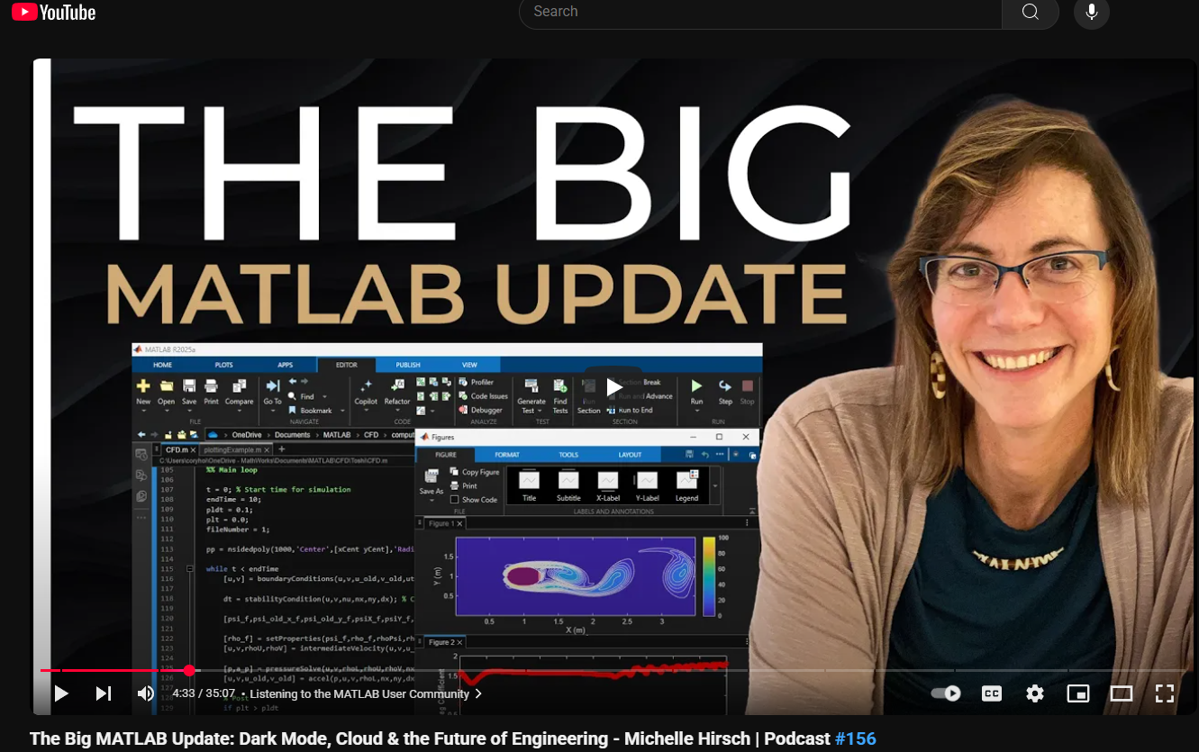
- Learn how dark theme may impacts charts and apps
- Discover best practices for theme-adaptive workflows
- Step-by-step examples for both script-based plots and advanced custom charts and UI components
- Discover new tools like ThemeChangedFcn, getTheme, and fliplightness