搜索
In just two weeks, the competition has become both intense and friendly as participants race to climb the team leaderboard, especially in Team Creative, where @Mehdi Dehghan currently leads with 1400+ points, followed by @Vasilis Bellos with 900+ points.
There’s still plenty of time to participate before the contest's main round ends on December 7. Solving just one problem in the contest problem group gives you a chance to win MathWorks T-shirts or socks. Completing the entire problem group not only boosts your odds but also helps your team win.
🎉 Week 2 Winners:
Weekly Prizes for Contest Problem Group Finishers:
@Cephas, @Athi, @Bin Jiang, @Armando Longobardi, @Simone, @Maxi, @Pietro, @Hong Son, @Salvatore, @KARUPPASAMYPANDIYAN M
Weekly Prizes for Contest Problem Group Solvers:
Weekly Prizes for Tips & Tricks Articles:
This week’s prize goes to @Athi for the highly detailed post Solving Systematically The Clueless - Lord Ned in the Game Room.
Comment from the judge:
Shortly after the problem set dropped, several folks recognized that the final problem, "Clueless", was a step above the rest in difficulty. So, not surprisingly, there were a few posts in the discussion boards related to how to tackle this problem. Athi, of the Cool Coders, really dug deep into how the rules and strategies could be turned into an algorithm. There's always more than one way to tackle any difficult programming problem, so it was nice to see some discussion in the comments on different ways you can structure the array that represents your knowledge of who has which cards.
Congratulations to all Week 2 winners! Let’s keep the momentum going!
In https://www.mathworks.com/matlabcentral/answers/38165-how-to-remove-decimal#comment_3345149 @Luisa asks,
@Cody Team, how can I vote or give a like in great comments?
It seems that there are not such options.
Developing an application in MATLAB often feels like a natural choice: it offers a unified environment, powerful visualization tools, accessible syntax, and a robust technical ecosystem. But when the goal is to build a compilable, distributable app, the path becomes unexpectedly difficult if your workflow depends on symbolic functions like sym, zeta, or lambertw.
This isn’t a minor technical inconvenience—it’s a structural contradiction. MATLAB encourages the creation of graphical interfaces, input validation, and dynamic visualization. It even provides an Application Compiler to package your code. But the moment you invoke sym, the compiler fails. No clear warning. No workaround. Just: you cannot compile. The same applies to zeta and lambertw, which rely on the symbolic toolbox.
So we’re left asking: how can a platform designed for scientific and technical applications block compilation of functions that are central to those very disciplines?
What Are the Alternatives?
- Rewrite everything numerically, avoiding symbolic logic—often impractical for advanced mathematical workflows.
- Use partial workarounds like matlabFunction, which may work but rarely preserve the original logic or flexibility.
- Switch platforms (e.g., Python with SymPy, Julia), which means rebuilding the architecture and leaving behind MATLAB’s ecosystem.
So, Is MATLAB Still Worth It?
That’s the real question. MATLAB remains a powerful tool for prototyping, teaching, analysis, and visualization. But when it comes to building compilable apps that rely on symbolic computation, the platform imposes limits that contradict its promise.
Is it worth investing time in a MATLAB app if you can’t compile it due to essential mathematical functions? Should MathWorks address this contradiction? Or is it time to rethink our tools?
I’d love to hear your thoughts. Is MATLAB still worth it for serious application development?
In just one week, we have hit an amazing milestone: 500+ players registered and 5000+ solutions submitted! We’ve also seen fantastic Tips & Tricks articles rolling in, making this contest a true community learning experience.
And here’s the best part: you don’t need to be a top-ranked player to win. To encourage more casual and first-time players to jump in, we’re introducing new weekly prizes starting Week 2!
New Casual Player Prizes:
- 5 extra MathWorks T-shirts or socks will be awarded every week.
- All you need to qualify is to register and solve one problem in the Contest Problem Group.
Jump in, try a few problems, and don’t be shy to ask questions in your team’s channel. You might walk away with a prize!
Week 1 Winners:
Weekly Prizes for Contest Problem Group Finishers:
@Mazhar, @Julien, @Mohammad Aryayi, @Pawel, @Mehdi Dehghan, @Christian Schröder, @Yolanda, @Dev Gupta, @Tomoaki Takagi, @Stefan Abendroth
Weekly Prizes for Tips & Tricks Articles:
We had a lot of people share useful tips (including some personal favorite MATLAB tricks). But Vasilis Bellos went *deep* into the Bridges of Nedsburg problem. Fittingly for a Creative Coder, his post was innovative and entertaining, while also cleverly sneaking in some hints on a neat solution method that wasn't advertised in the problem description.
Congratulations to all Week 1 winners! Prizes will be awarded after the contest ends. Let’s keep the momentum going!

It’s exciting to dive into a new dataset full of unfamiliar variables but it can also be overwhelming if you’re not sure where to start. Recently, I discovered some new interactive features in MATLAB live scripts that make it much easier to get an overview of your data. With just a few clicks, you can display sparklines and summary statistics using table variables, sort and filter variables, and even have MATLAB generate the corresponding code for reproducibility.
The Graphics and App Building blog published an article that walks through these features showing how to explore, clean, and analyze data—all without writing any code.
If you’re interested in streamlining your exploratory data analysis or want to see what’s new in live scripts, you might find it helpful:
If you’ve tried these features or have your own tips for quick data exploration in MATLAB, I’d love to hear your thoughts!
What a fantastic start to Cody Contest 2025! In just 2 days, over 300 players joined the fun, and we already have our first contest group finishers. A big shoutout to the first finisher from each team:
- Team Creative Coders: @Mehdi Dehghan
- Team Cool Coders: @Pawel
- Team Relentless Coders: @David Hill
- 🏆 First finisher overall: Mehdi Dehghan
Other group finishers: @Bin Jiang (Relentless), @Mazhar (Creative), @Vasilis Bellos (Creative), @Stefan Abendroth (Creative), @Armando Longobardi (Cool), @Cephas (Cool)
Kudos to all group finishers! 🎉
Reminder to finishers: The goal of Cody Contest is learning together. Share hints (not full solutions) to help your teammates complete the problem group. The winning team will be the one with the most group finishers — teamwork matters!
To all players: Don’t be shy about asking for help! When you do, show your work — include your code, error messages, and any details needed for others to reproduce your results.
Keep solving, keep sharing, and most importantly — have fun!
If you have solved a Cody problem before, you have likely seen the Scratch Pad text field below the Solution text field. It provides a quick way to get feedback on your solution before submitting it. Since submitting a solution takes you to a new page, any time a wrong solution is submitted, you have to navigate back to the problem page to try it again.
Instead, I use the Scratch Pad to test my solution repeatedly before submitting. That way, I get to a working solution faster without having to potentially go back and forth many times between the problem page and the wrong-solution page.
Here is my approach:
- Write a tentative solution.
- Copy a test case from the test suite into the Scratch Pad.
- Click the Run Function button—this is immediately below the Scratch Pad and above the Output panel and Submit buttons.
- If the solution does not work, modify the solution code, sometimes putting in disp() lines and/or removing semicolons to trace what the code is doing. Repeat until the solution passes.
- If the solution does work, repeat steps 2 through 4.
- Once there are no more test cases to copy and paste, clean up the code, if necessary (delete disp lines, reinstate all semicolons to suppress output). Click the Run Function button once more, just to make sure I did not break the solution while cleaning it up. Then, click the Submit button.
For problems with large test suites, you may find it useful to copy and paste in multiple test cases per iteration.
Hopefully you find this useful.
Title: Looking for Internship Guidance as a Beginner MATLAB/Simulink Learner
Hello everyone,
I’m a Computer Science undergraduate currently building a strong foundation in MATLAB and Simulink. I’m still at a beginner level, but I’m actively learning every day and can work confidently once I understand the concepts. Right now I’m focusing on MATLAB modeling, physics simulation, and basic control systems so that I can contribute effectively to my current project.
I’m part of an Autonomous Underwater Vehicle (AUV) team preparing for the Singapore AUV Challenge (SAUVC). My role is in physics simulation, controls, and navigation, and MATLAB/Simulink plays a major role in that pipeline. I enjoy physics and mathematics deeply, which makes learning modeling and simulation very exciting for me.
On the coding side, I practice competitive programming regularly—
• Codeforces rating: ~1200
• LeetCode rating: ~1500
So I'm comfortable with logic-building and problem solving. What I’m looking for:
I want to know how a beginner like me can start applying for internships related to MATLAB, Simulink, modeling, simulation, or any engineering team where MATLAB is widely used (including companies outside MathWorks).
I would really appreciate advice from the community on:
- What skills should I strengthen first?
- Which MATLAB/Simulink toolboxes are most important for beginners aiming toward simulation/control roles?
- What small projects or portfolio examples should I build to improve my profile?
- What is the best roadmap to eventually become a good candidate for internships in this area?
Any guidance, resources, or suggestions would be extremely helpful for me.
Thank you in advance to everyone who shares their experience!
The main round of Cody Contest 2025 kicks off today! Whether you’re a beginner or a seasoned solver, now’s your time to shine.
Here’s how to join the fun:
- Pick your team — choose one that matches your coding personality.
- Solve Cody problems — gain points and climb the leaderboard.
- Finish the Contest Problem Group — help your team win and unlock chances for weekly prizes by finishing the Cody Contest 2025 problem group.
- Share Tips & Tricks — post your insights to win a coveted MathWorks Yeti Bottle.
- Bonus Round — 2 players from each team will be invited to a fun live code-along event!
- Watch Party – join the big watch event to see how top players tackle Cody problems
Contest Timeline:
- Main Round: Nov 10 – Dec 7, 2025
- Bonus Round: Dec 8 – Dec 19, 2025
Big prizes await — MathWorks swag, Amazon gift cards, and shiny virtual badges!
We look forward to seeing you in the contest — learn, compete, and have fun!
Parallel Computing Onramp is here! This free, one-hour self-paced course teaches the basics of running MATLAB code in parallel using multiple CPU cores, helping users speed up their code and write code that handles information efficiently.
Remember, Onramps are free for everyone - give the new course a try if you're curious. Let us know what you think of it by replying below.
From my experience, MATLAB's Deep Learning Toolbox is quite user-friendly, but it still falls short of libraries like PyTorch in many respects. Most users tend to choose PyTorch because of its flexibility, efficiency, and rich support for many mathematical operators. In recent years, the number of dlarray-compatible mathematical functions added to the toolbox has been very limited, which makes it difficult to experiment with many custom networks. For example, svd is currently not supported for dlarray inputs.
This link (List of Functions with dlarray Support - MATLAB & Simulink) lists all functions that support dlarray as of R2026a — only around 200 functions (including toolbox-specific ones). I would like to see support for many more fundamental mathematical functions so that users have greater freedom when building and researching custom models. For context, the core MATLAB mathematics module contains roughly 600 functions, and many application domains build on that foundation.
I hope MathWorks will prioritize and accelerate expanding dlarray support for basic math functions. Doing so would significantly increase the Deep Learning Toolbox's utility and appeal for researchers and practitioners.
Thank you.
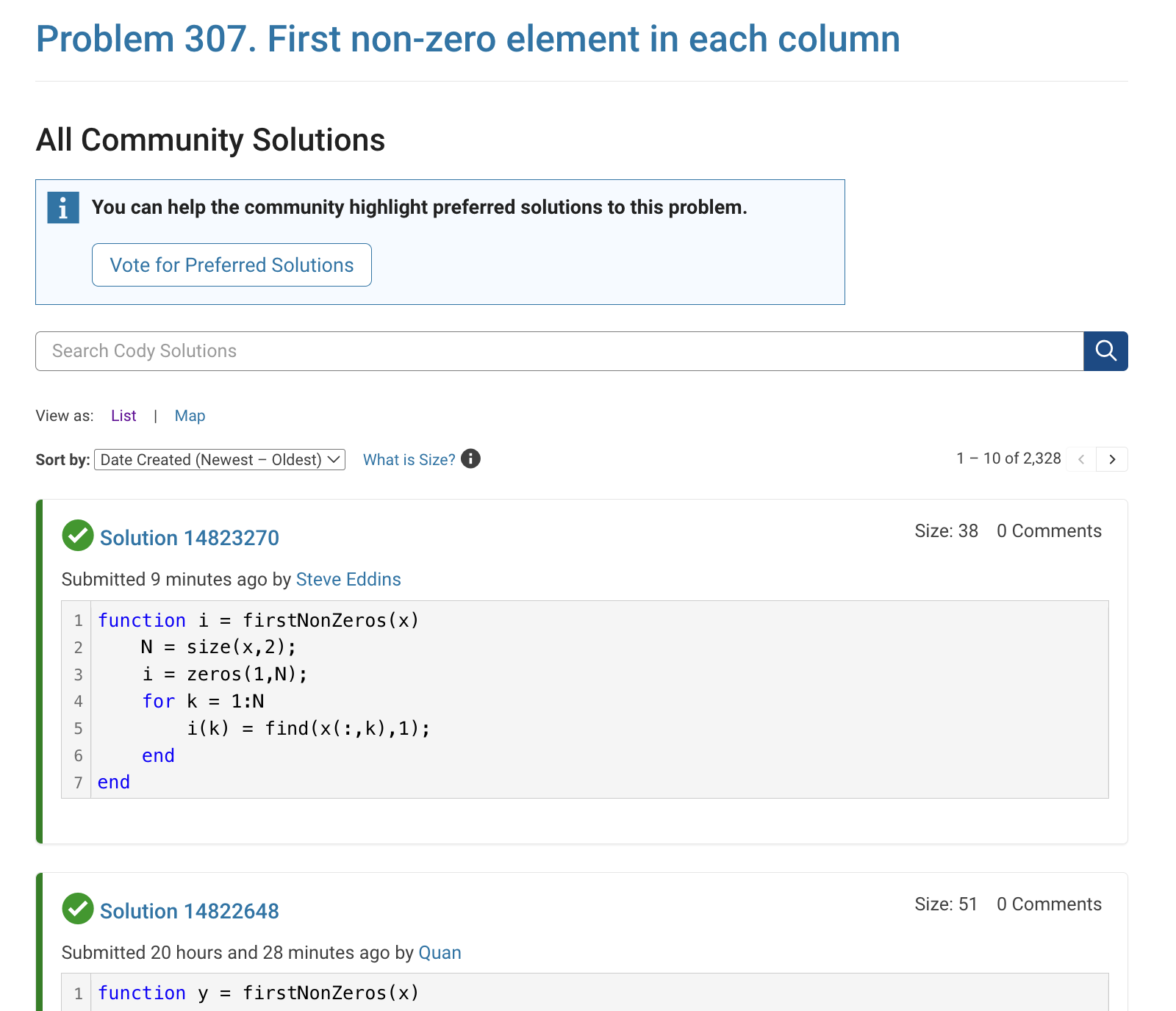
The all-community-solutions view shows the ID of each solution, and you can click on the link to go to the solution.
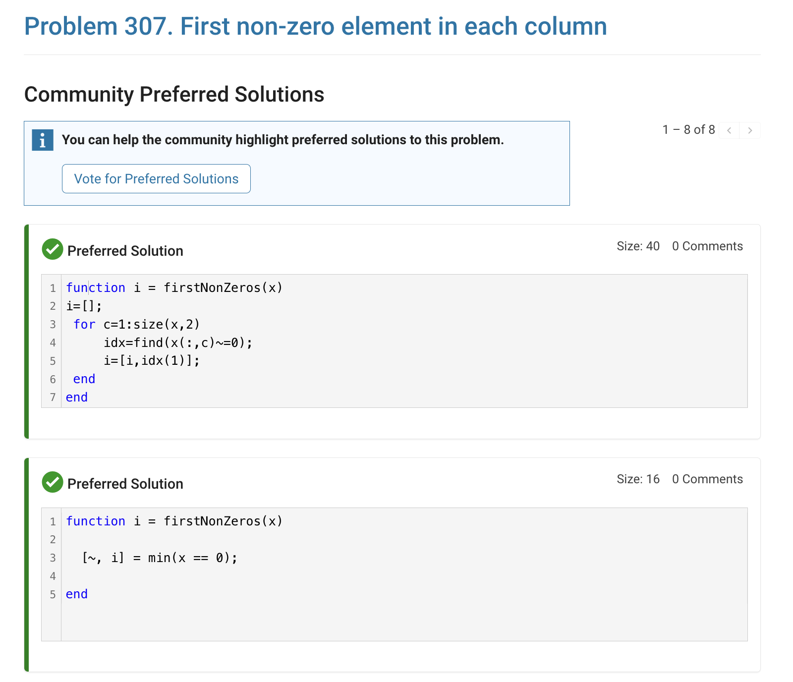
The preferred-community-solutions view does not show the solution IDs and does not link to the solutions. As far as I can tell, there is no way to get from that view to the solutions. If, for example, you want to go to the solution to leave a comment there, you can't.
All-community-solutions view:
Preferred-community-solutions view, with no solution IDs and no links:
Hi cody fellows,
I already solved more than 500 problems -months ago, last july if I remember well- and get this scholar badge, but then it suddenly disappeared a few weeks later. I then solved a few more problems and it reappeared.
Now I observed it disappeared once more a few days ago.
Have you also noticed this erratic behavior of the scholar badge ? Is it normal and / or intentional ? If not, how to explain it ? (deleted problems ?)
Cheers,
Nicolas
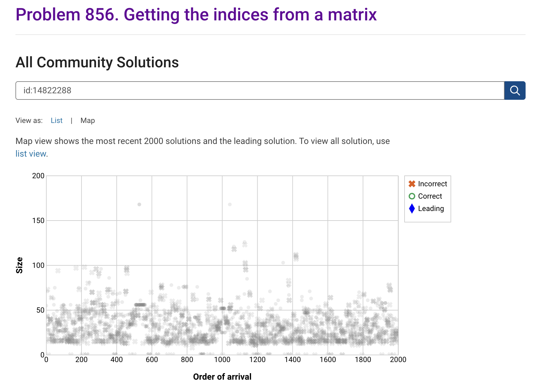
I'm seeing solution maps shown with low-contrast gray colors instead of the correct symbol colors. I have observed this using both Safari and Chrome. Screenshot:
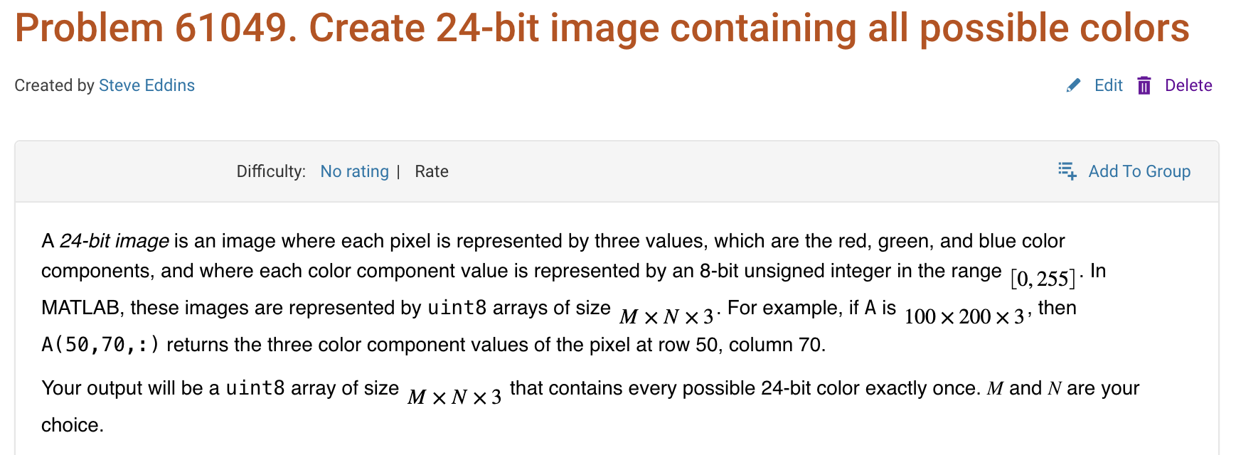
Here is a screenshot of a Cody problem that I just created. The math rendering is poor. (I have since edited the problem to remove the math formatting.)
I am excited to join this community to learn the more particularly the Matlab/Simulink
I just learned you can access MATLAB Online from the following shortcut in your web browser: https://matlab.new
Thanks @Yann Debray
From his recent blog post: pip & uv in MATLAB Online » Artificial Intelligence - MATLAB & Simulink
I'm developing a comprehensive MATLAB programming course and seeking passionate co-trainers to collaborate!
Why MATLAB Matters:Many people underestimate MATLAB's significance in:
- Communication systems
- Signal processing
- Mathematical modeling
- Engineering applications
- Scientific computing
Course Structure:
- Foundation Module: MATLAB basics and fundamentals
- Image Processing: Practical applications and techniques
- Signal Processing: Analysis and implementation
- Machine Learning: ML algorithms using MATLAB
- Hands-on Learning: Projects, assignments.
What I'm Looking For:
- Enthusiastic educators willing to share knowledge
- Experience in any MATLAB application area
- Commitment to collaborative teaching
Interested in joining as a co-trainer? Please comment below or reach out directly!
Are there any code restrictions for programming Cody solutions? I could not find anything mentioned at https://www.mathworks.com/matlabcentral/content/cody/about.html, other than toolbox functions not being available.
Online Doc + System Browser
11%
Online Doc + Dedicated Browser
11%
Offline Doc +System Browser
11%
Offline Doc + Dedicated Browser
23%
Hybrid Approach (Support All Modes)
23%
User-Definable / Fully Configurable
20%
35 个投票