搜索
’d like to share a complete MATLAB script that demonstrates how to compute and validate planetary masses from NASA JPL Horizons ephemeris data using the NKTg law (a conserved dynamic quantity). The result shows excellent agreement with the official mass values.
🔍 Background
In orbital mechanics, the NKTg quantity is defined as:
NKTg1 = x ⋅ p = x ⋅ (m ⋅ v)
Assuming conservation of NKTg during planetary motion, we derive an expression for mass:
m = NKTg1 / (x ⋅ v)
where:
x is orbital position (distance from Sun, m) v is orbital velocity (m/s) m is planetary mass (kg) p = m ⋅ v is linear momentum
We compare this interpolated mass with NASA JPL Horizons mass data.
🧾 MATLAB Code
matlab
%% NKTg Law – Planetary Mass Interpolation
% Data: NASA JPL Horizons (30–31/12/2024)
clear; clc;
%% Planet names
planet = {
'Mercury'
'Venus'
'Earth'
'Mars'
'Jupiter'
'Saturn'
'Uranus'
'Neptune'
};
%% Position x (km)
x_km = [
6.9817930e7
1.0893900e8
1.4710000e8
2.4923000e8
8.1662000e8
1.5065300e9
3.0013900e9
4.5589000e9
];
%% Velocity v (km/s)
v_kms = [
38.86
35.02
29.29
24.07
13.06
9.69
6.80
5.43
];
%% NASA masses m (kg)
m_nasa = [
3.301e23
4.867e24
5.972e24
6.417e23
1.898e27
5.683e26
8.681e25
1.024e26
];
%% Unit conversion
x = x_km * 1e3; % km → m
v = v_kms * 1e3; % km/s → m/s
%% Linear momentum
p = m_nasa .* v; % kg·m/s
%% NKTg1 computation
NKTg1 = x .* p; % NKTm
%% Mass interpolation from NKTg law
% m = NKTg1 / (x · v)
m_interp = NKTg1 ./ (x .* v);
%% Mass difference
delta_m = m_nasa - m_interp;
%% Display results
T = table(planet, x_km, v_kms, NKTg1, m_interp, m_nasa, delta_m, ...
'VariableNames', {
'Planet', 'x_km', 'v_km_s', 'NKTg1_NKTm', ...
'Interpolated_m_kg', 'NASA_m_kg', 'Delta_m_kg'
});
disp(T);
📊 Results
After running the script, you’ll see a table listing:
| Planet | x (km) | v (km/s) | NKTg1 | Interpolated m | NASA mass | Δ mass |
The interpolated masses match NASA masses extremely closely (differences extremely small), showing that the NKTg formulation preserves mass consistency.
💡 Notes
✔ Orbital data (position, velocity) are taken from NASA JPL Horizons ✔ Units are carefully converted (km → m) ✔ The NKTg law interprets dynamic invariants
❓ Questions for the community
Has anyone applied this technique to asteroids, comets, or spacecraft flybys? Could this NKTg approach suggest alternative invariant quantities in orbital mechanics? Suggestions for numerical stability improvements?
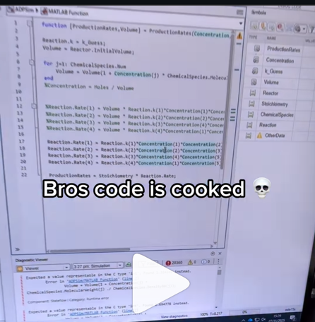
A coworker shared with me a hilarious Instagram post today. A brave bro posted a short video showing his MATLAB code… casually throwing 49,000 errors!
Surprisingly, the video went virial and recieved 250,000+ likes and 800+ comments. You really never know what the Instagram algorithm is thinking, but apparently “my code is absolutely cooked” is a universal developer experience 😂
Last note: Can someone please help this Bro fix his code?
I’d like to share a compact MATLAB example showing how a variable-inertia formulation (called the NKTg Law) can be evaluated using publicly available NASA Neptune orbital data.
This work focuses on a simple, reproducible MATLAB workflow for evaluating a variable-inertia formulation using public data.
using a simple, transparent MATLAB workflow.Model Definition
p = m * v; % linear momentum
NKTg1 = x * p;
% position–momentum interaction
NKTg2 = dm_dt * p;
% mass-variation–momentum interaction
NKTg =
sqrt(NKTg1^2 + NKTg2^2);
This formulation evaluates the state tendency of a system with position x, velocity v, and mass variation dm/dt.MATLAB NeptuneNKTg Law Verification using NASA Neptune Data
Author: Nguyen Khanh Tung
Purpose: Verify NKTg Law with Neptune data (2023–2024)
clc; clear; format long e;
% Constants & Initial Parameters
v =
5.43e3; % Velocity (m/s) (5.43 km/s)
dm_dt =
-2.0e-5; % Mass loss rate (kg/s)
% Time vector (seconds from start of year, approx)
t = [
0 90 180 270 365] * 24 * 3600;
% NASA 2023 Data
x_2023_km = [ ...
4498396440
4503443661
4553946490
4503443661
4498396440 ];
m_2023 = [ ...
1.02430000e26
1.02429980e26
1.02429960e26
1.02429940e26
1.02429920e26 ];
% Convert km → m
x_2023 = x_2023_km *
1e3;
% NKTg Core Calculations (2023)
p_2023 = m_2023 .* v;
% Momentum
NKTg1_2023 = x_2023 .* p_2023;
% x · p
NKTg2_2023 = dm_dt .* p_2023;
% (dm/dt) · p
NKTg_2023 =
sqrt(NKTg1_2023.^2 + NKTg2_2023.^2);
% Simulated 2024 Mass (NKTg Law)
m_2024 = m_2023(
1) + dm_dt .* t;
p_2024 = m_2024 .* v;
x_2024 = x_2023;
% Orbit assumed stable (NASA-confirmed)
NKTg1_2024 = x_2024 .* p_2024;
NKTg2_2024 = dm_dt .* p_2024;
NKTg_2024 =
sqrt(NKTg1_2024.^2 + NKTg2_2024.^2);
% Relative Mass Error vs NASA
m_NASA_2024 =
1.02430000e26 * ones(size(m_2024));
relative_error =
abs(m_2024 - m_NASA_2024) ./ m_NASA_2024 * 100;
% Display Results
disp('==== NKTg Law Verification (Neptune 2024) ====')
table(x_2024/1e3, m_2024, m_NASA_2024, relative_error, ...
'VariableNames', ...
{
'Position_km','Mass_NKTg_kg','Mass_NASA_kg','Relative_Error_%'})
% Plot Results
figure;
plot(t/86400, m_2024, 'LineWidth', 2); hold on;
plot(t/86400, m_NASA_2024, '--', 'LineWidth', 2);
xlabel(
'Days in 2024');
ylabel(
'Mass (kg)');
title(
'Neptune Mass Evolution: NKTg vs NASA');
legend('NKTg Simulation','NASA Constant Mass');
grid on;
figure;
plot(t/86400, NKTg_2024, 'LineWidth', 2);
xlabel(
'Days in 2024');
ylabel(
'NKTg');
title(
'Total NKTg Stability Over Time');
grid on;
Observation
- With an ultra-small mass variation, orbital position and velocity remain unchanged, consistent with NASA data.
- The NKTg formulation remains numerically stable.
- This makes it suitable for simulation, control, or sensitivity analysis, rather than orbit prediction itself.
Notes
- Motion is treated in 1D heliocentric distance for simplicity.
- dm/dt is an illustrative parameter, not a measured physical loss.
- Full datasets and extended verification are available externally if needed.
Happy to hear thoughts from the MATLAB community — especially regarding:
- extending this to 3D state vectors
- numerical conditioning
- comparison with classical invariants
Thanks!
Currently, the open-source MATLAB Community is accessed via the desktop web interface, and the experience on mobile devices is not very good—especially switching between sections like Discussion, FEX, Answers, and Cody is awkward. Having a dedicated app would make using the community much more convenient on phones.
Similarty,github has Mobile APP, It's convient for me.
Is it possible to display a variable value within the ThingSpeak plot area?
https://www.mathworks.com/matlabcentral/answers/2182045-why-can-t-i-renew-or-purchase-add-ons-for-m…
"As of January 1, 2026, Perpetual Student and Home offerings have been sunset and replaced with new Annual Subscription Student and Home offerings."
So, Perpetual licenses for Student and Home versions are no more. Also, the ability for Student and Home to license just MATLAB by itself has been removed.
The new offering for Students is $US119 per year with no possibility of renewing through a Software Maintenance Service type offering. That $US119 covers the Student Suite of MATLAB and Simulink and 11 other toolboxes. Before, the perpetual license was $US99... and was a perpetual license, so if (for example) you bought it in second year you could use it in third and fourth year for no additional cost. $US99 once, or $US99 + $US35*2 = $US169 (if you took SMS for 2 years) has now been replaced by $US119 * 3 = $US357 (assuming 3 years use.)
The new offering for Home is $US165 per year for the Suite (MATLAB + 12 common toolboxes.) This is a less expensive than the previous $US150 + $US49 per toolbox if you had a use for those toolboxes . Except the previous price was a perpetual license. It seems to me to be more likely that Home users would have a use for the license for extended periods, compared to the Student license (Student licenses were perpetual licenses but were only valid while you were enrolled in degree granting instituations.)
Unfortunately, I do not presently recall the (former) price for SMS for the Home license. It might be the case that by the time you added up SMS for base MATLAB and the 12 toolboxes, that you were pretty much approaching $US165 per year anyhow... if you needed those toolboxes and were willing to pay for SMS.
But any way you look at it, the price for the Student version has effectively gone way up. I think this is a bad move, that will discourage students from purchasing MATLAB in any given year, unless they need it for courses. No (well, not much) more students buying MATLAB with the intent to explore it, knowing that it would still be available to them when it came time for their courses.
You may have come across code that looks like that in some languages:
stubFor(get(urlPathEqualTo("/quotes"))
.withHeader("Accept", equalTo("application/json"))
.withQueryParam("s", equalTo(monitoredStock))
.willReturn(aResponse())
.withStatus(200)
.withHeader("Content-Type", "application/json")
.withBody("{\\"symbol\\": \\"XYZ\\", \\"bid\\": 20.2, " + "\\"ask\\": 20.6}")))
That’s Java. Even if you can’t fully decipher it, you can get a rough idea of what it is supposed to do, build a rather complex API query.
Or you may be familiar with the following similar and frequent syntax in Python:
import seaborn as sns
sns.load_dataset('tips').sample(10, random_state=42).groupby('day').mean()
Here’s is how it works: multiple method calls are linked together in a single statement, spanning over one or several lines, usually because each method returns the same object or another object that supports further calls.
That technique is called method chaining and is popular in Object-Oriented Programming.
A few years ago, I looked for a way to write code like that in MATLAB too. And the answer is that it can be done in MATLAB as well, whevener you write your own class!
Implementing a method that can be chained is simply a matter of writing a method that returns the object itself.
In this article, I would like to show how to do it and what we can gain from such a syntax.
Example
A few years ago, I first sought how to implement that technique for a simulation launcher that had lots of parameters (far too many):
lauchSimulation(2014:2020, true, 'template', 'TmplProd', 'Priority', '+1', 'Memory', '+6000')
As you can see, that function takes 2 required inputs, and 3 named parameters (whose names aren’t even consistent, with ‘Priority’ and ‘Memory’ starting with an uppercase letter when ‘template’ doesn’t).
(The original function had many more parameters that I omit for the sake of brevity. You may also know of such functions in your own code that take a dozen parameters which you can remember the exact order.)
I thought it would be nice to replace that with:
SimulationLauncher() ...
.onYears(2014:2020) ...
.onDistributedCluster() ... % = equivalent of the previous "true"
.withTemplate('TmplProd') ...
.withPriority('+1') ...
.withReservedMemory('+6000') ...
.launch();
The first 6 lines create an object of class SimulationLauncher, calls several methods on that object to set the parameters, and lastly the method launch() is called, when all desired parameters have been set.
To make it cleared, the syntax previously shown could also be rewritten as:
launcher = SimulationLauncher();
launcher = launcher.onYears(2014:2020);
launcher = launcher.onDistributedCluster();
launcher = launcher.withTemplate('TmplProd');
launcher = launcher.withPriority('+1');
launcher = launcher.withReservedMemory('+6000');
launcher.launch();
Before we dive into how to implement that code, let’s examine the advantages and drawbacks of that syntax.
Benefits and drawbacks
Because I have extended the chained methods over several lines, it makes it easier to comment out or uncomment any one desired option, should the need arise. Furthermore, we need not bother any more with the order in which we set the parameters, whereas the usual syntax required that we memorize or check the documentation carefully for the order of the inputs.
More generally, chaining methods has the following benefits and a few drawbacks:
Benefits:
- Conciseness: Code becomes shorter and easier to write, by reducing visual noise compared to repeating the object name.
- Readability: Chained methods create a fluent, human-readable structure that makes intent clear.
- Reduced Temporary Variables: There's no need to create intermediary variables, as the methods directly operate on the object.
Drawbacks:
- Debugging Difficulty: If one method in a chain fails, it can be harder to isolate the issue. It effectively prevents setting breakpoints, inspecting intermediate values, and identifying which method failed.
- Readability Issues: Overly long and dense method chains can become hard to follow, reducing clarity.
- Side Effects: Methods that modify objects in place can lead to unintended side effects when used in long chains.
Implementation
In the SimulationLauncher class, the method lauch performs the main operation, while the other methods just serve as parameter setters. They take the object as input and return the object itself, after modifying it, so that other methods can be chained.
classdef SimulationLauncher
properties (GetAccess = private, SetAccess = private)
years_
isDistributed_ = false;
template_ = 'TestTemplate';
priority_ = '+2';
memory_ = '+5000';
end
methods
function varargout = launch(obj)
% perform whatever needs to be launched
% using the values of the properties stored in the object:
% obj.years_
% obj.template_
% etc.
end
function obj = onYears(obj, years)
assert(isnumeric(years))
obj.years_ = years;
end
function obj = onDistributedCluster(obj)
obj.isDistributed_ = true;
end
function obj = withTemplate(obj, template)
obj.template_ = template;
end
function obj = withPriority(obj, priority)
obj.priority_ = priority;
end
function obj = withMemory( obj, memory)
obj.memory_ = memory;
end
end
end
As you can see, each method can be in charge of verifying the correctness of its input, independantly. And what they do is just store the value of parameter inside the object. The class can define default values in the properties block.
You can configure different launchers from the same initial object, such as:
launcher = SimulationLauncher();
launcher = launcher.onYears(2014:2020);
launcher1 = launcher ...
.onDistributedCluster() ...
.withReservedMemory('+6000');
launcher2 = launcher ...
.withTemplate('TmplProd') ...
.withPriority('+1') ...
.withReservedMemory('+7000');
If you call the same method several times, only the last recorded value of the parameter will be taken into acount:
launcher = SimulationLauncher();
launcher = launcher ...
.withReservedMemory('+6000') ...
.onDistributedCluster() ...
.onYears(2014:2020) ...
.withReservedMemory('+7000') ...
.withReservedMemory('+8000');
% The value of "memory" will be '+8000'.
If the logic is still not clear to you, I advise you play a bit with the debugger to better understand what’s going on!
Conclusion
I love how the method chaining technique hides the minute detail that we don’t want to bother with when trying to understand what a piece of code does.
I hope this simple example has shown you how to apply it to write and organise your code in a more readable and convenient way.
Let me know if you have other questions, comments or suggestions. I may post other examples of that technique for other useful uses that I encountered in my experience.
I struggle with animations. I often want a simple scrollable animation and wind up having to export to some external viewer in some supported format. The new Live Script automation of animations fails and sabotages other methods and it is not well documented so even AIs are clueless how to resolve issues. Often an animation works natively but not with MATLAB Online. Animation of results seems to me rather basic and should be easier!
Frequently, I find myself doing things like the following,
xyz=rand(100,3);
XYZ=num2cell(xyz,1);
scatter3(XYZ{:,1:3})
But num2cell is time-consuming, not to mention that requiring it means extra lines of code. Is there any reason not to enable this syntax,
scatter3(xyz{:,1:3})
so that I one doesn't have to go through num2cell? Here, I adopt the rule that only dimensions that are not ':' will be comma-expanded.
I’m currently developing a multi-platform viewer using Flutter to eliminate the hassle of manual channel setup. Instead of adding IDs one by one, the app uses your User API Key to automatically discover and list all your ThingSpeak channels instantly.
Key Highlights (Work in Progress):
- Automatic Sync: All your channels appear in seconds.
- Multi-platform: Built for Web, Android, Windows, and Linux.
- Privacy-Focused: Secure local storage for your API keys.
If you use tables extensively to perform data analysis, you may at some point have wanted to add new functionalities suited to your specific applications. One straightforward idea is to create a new class that subclasses the built-in table class. You would then benefit from all inherited existing methods.
One workaround is to create a new class that wraps a table as a Property, and re-implement all the methods that you need and are already defined for table. The is not too difficult, except for the subsref method, for which I’ll provide the code below.
Class definition
Defining a wrapper of the table class is quite straightforward. In this example, I call the class “Report” because that is what I intend to use the class for, to compute and store reports. The constructor just takes a table as input:
classdef Rapport
methods
function obj = Report(t)
if isa(t, 'Report')
obj = t;
else
obj.t_ = t;
end
end
end
properties (GetAccess = private, SetAccess = private)
t_ table = table();
end
end
I designed the constructor so that it converts a table into a Report object, but also so that if we accidentally provide it with a Report object instead of a table, it will not generate an error.
Reproducing the behaviour of the table class
Implementing the existing methods of the table class for the Report class if pretty easy in most cases.
I made use of a method called “table” in order to be able to get the data back in table format instead of a Report, instead of accessing the property t_ of the object. That method can also be useful whenever you wish to use the methods or functions already existing for tables (such as writetable, rowfun, groupsummary…).
classdef Rapport
...
methods
function t = table(obj)
t = obj.t_;
end
function r = eq(obj1,obj2)
r = isequaln(table(obj1), table(obj2));
end
function ind = size(obj, varargin)
ind = size(table(obj), varargin{:});
end
function ind = height(obj, varargin)
ind = height(table(obj), varargin{:});
end
function ind = width(obj, varargin)
ind = width(table(obj), varargin{:});
end
function ind = end(A,k,n)
% ind = end(A.t_,k,n);
sz = size(table(A));
if k < n
ind = sz(k);
else
ind = prod(sz(k:end));
end
end
end
end
In the case of horzcat (same principle for vertcat), it is just a matter of converting back and forth between the table and Report classes:
classdef Rapport
...
methods
function r = horzcat(obj1,varargin)
listT = cell(1, nargin);
listT{1} = table(obj1);
for k = 1:numel(varargin)
kth = varargin{k};
if isa(kth, 'Report')
listT{k+1} = table(kth);
elseif isa(kth, 'table')
listT{k+1} = kth;
else
error('Input must be a table or a Report');
end
end
res = horzcat(listT{:});
r = Report(res);
end
end
end
Adding a new method
The plus operator already exists for the table class and works when the table contains all numeric values. It sums columns as long as the tables have the same length.
Something I think would be nice would be to be able to write t1 + t2, and that would perform an outerjoin operation between the tables and any sizes having similar indexing columns.
That would be so concise, and that's what we’re going to implement for the Report class as an example. That is called “plus operator overloading”. Of course, you could imagine that the “+” operator is used to compute something else, for example adding columns together with regard to the keys index. That depends on your needs.
Here’s a unittest example:
classdef ReportTest < matlab.unittest.TestCase
methods (Test)
function testPlusOperatorOverload(testCase)
t1 = array2table( ...
{ 'Smith', 'Male' ...
; 'JACKSON', 'Male' ...
; 'Williams', 'Female' ...
} , 'VariableNames', {'LastName' 'Gender'} ...
);
t2 = array2table( ...
{ 'Smith', 13 ...
; 'Williams', 6 ...
; 'JACKSON', 4 ...
}, 'VariableNames', {'LastName' 'Age'} ...
);
r1 = Report(t1);
r2 = Report(t2);
tRes = r1 + r2;
tExpected = Report( array2table( ...
{ 'JACKSON' , 'Male', 4 ...
; 'Smith' , 'Male', 13 ...
; 'Williams', 'Female', 6 ...
} , 'VariableNames', {'LastName' 'Gender' 'Age'} ...
) );
testCase.verifyEqual(tRes, tExpected);
end
end
end
And here’s how I’d implement the plus operator in the Report class definition, so that it also works if I add a table and a Report:
classdef Rapport
...
methods
function r = plus(obj1,obj2)
table1 = table(obj1);
table2 = table(obj2);
result = outerjoin(table1, table2 ...
, 'Type', 'full', 'MergeKeys', true);
r = reportingits.dom.Rapport(result);
end
end
end
The case of the subsref method
If we wish to access the elements of an instance the same way we would with regular tables, whether with parentheses, curly braces or directly with the name of the column, we need to implement the subsref and subsasgn methods. The second one, subsasgn is pretty easy, but subsref is a bit tricky, because we need to detect whether we’re directing towards existing methods or not.
Here’s the code:
classdef Rapport
...
methods
function A = subsasgn(A,S,B)
A.t_ = subsasgn(A.t_,S,B);
end
function B = subsref(A,S)
isTableMethod = @(m) ismember(m, methods('table'));
isReportMethod = @(m) ismember(m, methods('Report'));
switch true
case strcmp(S(1).type, '.') && isReportMethod(S(1).subs)
methodName = S(1).subs;
B = A.(methodName)(S(2).subs{:});
if numel(S) > 2
B = subsref(B, S(3:end));
end
case strcmp(S(1).type, '.') && isTableMethod (S(1).subs)
methodName = S(1).subs;
if ~isReportMethod(methodName)
error('The method "%s" needs to be implemented!', methodName)
end
otherwise
B = subsref(table(A),S(1));
if istable(B)
B = Report(B);
end
if numel(S) > 1
B = subsref(B, S(2:end));
end
end
end
end
end
Conclusion
I believe that the table class is Sealed because is case new methods are introduced in MATLAB in the future, the subclass might not be compatible if we created any or generate unexpected complexity.
The table class is a really powerful feature.
I hope this example has shown you how it is possible to extend the use of tables by adding new functionalities and maybe given you some ideas to simplify some usages. I’ve only happened to find it useful in very restricted cases, but was still happy to be able to do so.
In case you need to add other methods of the table class, you can see the list simply by calling methods(’table’).
Feel free to share your thoughts or any questions you might have! Maybe you’ll decide that doing so is a bad idea in the end and opt for another solution.
(Requested for newer MATLAB releases (e.g. R2026B), MATLAB Parallel Processing toolbox.)
Lower precision array types have been gaining more popularity over the years for deep learning. The current lowest precision built-in array type offered by MATLAB are 8-bit precision arrays, e.g. int8 and uint8. A good thing is that these 8-bit array types do have gpuArray support, meaning that one is able to design GPU MEX codes that take in these 8-bit arrays and reinterpret them bit-wise as other 8-bit array types, e.g. FP8, which is especially common array type used in modern day deep learning applications. I myself have used this to develop forward pass operations with 8-bit precision that are around twice as fast as 16-bit operations and with output arrays that still agree well with 16-bit outputs (measured with high cosine similarity). So the 8-bit support that MATLAB offers is already quite sufficient.
Recently, 4-bit precision array types have been shown also capable of being very useful in deep learning. These array types can be processed with Tensor Cores of more modern GPUs, such as NVIDIA's Blackwell architecture. However, MATLAB does not yet have a built-in 4-bit precision array type.
Just like MATLAB has int8 and uint8, both also with gpuArray support, it would also be nice to have MATLAB have int4 and uint4, also with gpuArray support.
The Cody Contest 2025 has officially wrapped up! Over the past 4 weeks, more than 700 players submitted over 20,000 solutions. In addition, participants shared 20+ high-quality Tips & Tricksarticles—resources that will benefit Cody users for years to come.
Now it’s time to announce the winners.
🎉 Week 4 winners:
Weekly Prizes for Contest Problem Group Finishers:
@JKMSMKJ, @Yu Zhang, @Oliver Jaros, @Pauli Huusari, @Karl, @Marcos Silveira, @goc3, @Ildeberto de los Santos Ruiz, @Norberto, @Eric
Weekly Prizes for Contest Problem Group Solvers:
Weekly Prizes for Tips & Tricks Articles:
This week’s prize goes to @WANG Zi-Xiang. See the comments from our judge and problem group author @Matt Tearle:
‘We had a lot of great tips for solving Cody problems in general and the contest problems specifically. But we all know there are those among us who, having solved the problem, still want to tinker and make their code better. There are different definitions of "better", but code size remains the base metric in Cody. Enter Wang Zi-Xiang who compiled a list of many tips for reducing Cody size. This post also generated some great discussion (even prompting our insane autocrat, Lord Ned himself, to chime in). I particularly like the way that, while reducing Cody size often requires some arcane tricks that would normally be considered bad coding practice, the intellectual activity of trying to "game the system" makes you consider different programming approaches, and sometimes leads you to learn corners of MATLAB that you didn't know.’
🏆 Grand Prizes for the Main Round
Team Relentless Coders:
2nd Place: @Roberto
Team Creative Coders:
Team Cool Coders
Congratulations to all! Securing a top position on the leaderboard requires not only advanced MATLAB skills but also determination and consistency throughout the four-week contest. You will receive Amazon gift cards.
🥇 Winning Team
The competition was incredibly tight—we even had to use the tie-breaker rule.
Both Team Cool Coders and Team Relentless Coders achieved 16 contest group finishers. However, the last finisher on Cool Coders completed the problem group at 1:02 PM on Dec 7, while the last finisher on Relentless Coders finished at 9:47 PM the same day.
Such a close finish! Congratulations to Team Cool Coders, who have earned the Winning Team Finishers badge.

🎬 Bonus Round
Invitations have been sent to the 6 players who qualified for the Bonus Round. Stay tuned for updates—including the Big Watch Party afterward!
Congratulations again to all winners! We’ll be reaching out after the contest ends. It has been an exciting, rewarding, and knowledge-packed journey.
See you next year!
I can't believe someone put time into this ;-)

Our exportgraphics and copygraphics functions now offer direct and intuitive control over the size, padding, and aspect ratio of your exported figures.
- Specify Output Size: Use the new Width, Height, and Units name-value pairs
- Control Padding: Easily adjust the space around your axes using the Padding argument, or set it to to match the onscreen appearance.
- Preserve Aspect Ratio: Use PreserveAspectRatio='on' to maintain the original plot proportions when specifying a fixed size.
- SVG Export: The exportgraphics function now supports exporting to the SVG file format.
Check out the full article on the Graphics and App Building blog for examples and details: Advanced Control of Size and Layout of Exported Graphics
No, staying home (or where I'm now)
25%
Yes, 1 night
0%
Yes, 2 nights
12.5%
Yes, 3 nights
12.5%
Yes, 4-7 nights
25%
Yes, 8 nights or more
25%
8 个投票
Hi everyone
I've been using ThingSpeak for several years now without an issue until last Thursday.
I have four ThingSpeak channels which are used by three Arduino devices (in two locations/on two distinct networks) all running the same code.
All three devices stopped being able to write data to my ThingSpeak channels around 17:00 CET on 4 Dec and are still unable to.
Nothing changed on this side, let alone something that would explain the problem.
I would note that data can still be written to all the channels via a browser so there is no fundamental problem with the channels (such as being full).
Since the above date and time, any HTTP/1.1 'update' (write) requests via the REST API (using both simple one-write GET requests or bulk JSON POST requests) are timing out after 5 seconds and no data is being written. The 5 second timeout is my Arduino code's default, but even increasing it to 30 seconds makes no difference. Before all this, responses from ThingSpeak were sub-second.
I have recompiled the Arduino code using the latest libraries and that didn't help.
I have tested the same code again another random api (api.ipify.org) and that works just fine.
Curl works just fine too, also usng HTTP/1.1
So the issue appears to be something particular to the combination of my Arduino code *and* the ThingSpeak environment, where something changed on the ThingSpeak end at the above date and time.
If anyone in the community has any suggestions as to what might be going on, I would greatly appreciate the help.
Peter
Over the past three weeks, players have been having great fun solving problems, sharing knowledge, and connecting with each other. Did you know over 15,000 solutions have already been submitted?
This is the final week to solve Cody problems and climb the leaderboard in the main round. Remember: solving just one problem in the contest problem group gives you a chance to win MathWorks T-shirts or socks.
🎉 Week 3 Winners:
Weekly Prizes for Contest Problem Group Finishers:
@Umar, @David Hill, @Takumi, @Nicolas, @WANG Zi-Xiang, @Rajvir Singh Gangar, @Roberto, @Boldizsar, @Abi, @Antonio
Weekly Prizes for Contest Problem Group Solvers:
Weekly Prizes for Tips & Tricks Articles:
This week’s prize goes to @Cephas. See the comments from our judge and problem group author @Matt Tearle:
'Some folks have posted deep dives into how to tackle specific problems in the contest set. But others have shared multiple smaller, generally useful tips. This week, I want to congratulate the cumulative contribution of Cool Coder Cephas, who has shared several of my favorite MATLAB techniques, including logical indexing, preallocation, modular arithmetic, and more. Cephas has also given some tips applying these MATLAB techniques to specific contest problems, such as using a convenient MATLAB function to vectorize the Leaderboard problem. Tip for Problem 61059 – Leaderboard for the Nedball World Cup:'
Congratulations to all Week 3 winners! Let’s carry this momentum into the final week!

The formula comes from @yuruyurau. (https://x.com/yuruyurau)
digital life 1

figure('Position',[300,50,900,900], 'Color','k');
axes(gcf, 'NextPlot','add', 'Position',[0,0,1,1], 'Color','k');
axis([0, 400, 0, 400])
SHdl = scatter([], [], 2, 'filled','o','w', 'MarkerEdgeColor','none', 'MarkerFaceAlpha',.4);
t = 0;
i = 0:2e4;
x = mod(i, 100);
y = floor(i./100);
k = x./4 - 12.5;
e = y./9 + 5;
o = vecnorm([k; e])./9;
while true
t = t + pi/90;
q = x + 99 + tan(1./k) + o.*k.*(cos(e.*9)./4 + cos(y./2)).*sin(o.*4 - t);
c = o.*e./30 - t./8;
SHdl.XData = (q.*0.7.*sin(c)) + 9.*cos(y./19 + t) + 200;
SHdl.YData = 200 + (q./2.*cos(c));
drawnow
end
digital life 2

figure('Position',[300,50,900,900], 'Color','k');
axes(gcf, 'NextPlot','add', 'Position',[0,0,1,1], 'Color','k');
axis([0, 400, 0, 400])
SHdl = scatter([], [], 2, 'filled','o','w', 'MarkerEdgeColor','none', 'MarkerFaceAlpha',.4);
t = 0;
i = 0:1e4;
x = i;
y = i./235;
e = y./8 - 13;
while true
t = t + pi/240;
k = (4 + sin(y.*2 - t).*3).*cos(x./29);
d = vecnorm([k; e]);
q = 3.*sin(k.*2) + 0.3./k + sin(y./25).*k.*(9 + 4.*sin(e.*9 - d.*3 + t.*2));
SHdl.XData = q + 30.*cos(d - t) + 200;
SHdl.YData = 620 - q.*sin(d - t) - d.*39;
drawnow
end
digital life 3

figure('Position',[300,50,900,900], 'Color','k');
axes(gcf, 'NextPlot','add', 'Position',[0,0,1,1], 'Color','k');
axis([0, 400, 0, 400])
SHdl = scatter([], [], 1, 'filled','o','w', 'MarkerEdgeColor','none', 'MarkerFaceAlpha',.4);
t = 0;
i = 0:1e4;
x = mod(i, 200);
y = i./43;
k = 5.*cos(x./14).*cos(y./30);
e = y./8 - 13;
d = (k.^2 + e.^2)./59 + 4;
a = atan2(k, e);
while true
t = t + pi/20;
q = 60 - 3.*sin(a.*e) + k.*(3 + 4./d.*sin(d.^2 - t.*2));
c = d./2 + e./99 - t./18;
SHdl.XData = q.*sin(c) + 200;
SHdl.YData = (q + d.*9).*cos(c) + 200;
drawnow; pause(1e-2)
end
digital life 4

figure('Position',[300,50,900,900], 'Color','k');
axes(gcf, 'NextPlot','add', 'Position',[0,0,1,1], 'Color','k');
axis([0, 400, 0, 400])
SHdl = scatter([], [], 1, 'filled','o','w', 'MarkerEdgeColor','none', 'MarkerFaceAlpha',.4);
t = 0;
i = 0:4e4;
x = mod(i, 200);
y = i./200;
k = x./8 - 12.5;
e = y./8 - 12.5;
o = (k.^2 + e.^2)./169;
d = .5 + 5.*cos(o);
while true
t = t + pi/120;
SHdl.XData = x + d.*k.*sin(d.*2 + o + t) + e.*cos(e + t) + 100;
SHdl.YData = y./4 - o.*135 + d.*6.*cos(d.*3 + o.*9 + t) + 275;
SHdl.CData = ((d.*sin(k).*sin(t.*4 + e)).^2).'.*[1,1,1];
drawnow;
end
digital life 5

figure('Position',[300,50,900,900], 'Color','k');
axes(gcf, 'NextPlot','add', 'Position',[0,0,1,1], 'Color','k');
axis([0, 400, 0, 400])
SHdl = scatter([], [], 1, 'filled','o','w',...
'MarkerEdgeColor','none', 'MarkerFaceAlpha',.4);
t = 0;
i = 0:1e4;
x = mod(i, 200);
y = i./55;
k = 9.*cos(x./8);
e = y./8 - 12.5;
while true
t = t + pi/120;
d = (k.^2 + e.^2)./99 + sin(t)./6 + .5;
q = 99 - e.*sin(atan2(k, e).*7)./d + k.*(3 + cos(d.^2 - t).*2);
c = d./2 + e./69 - t./16;
SHdl.XData = q.*sin(c) + 200;
SHdl.YData = (q + 19.*d).*cos(c) + 200;
drawnow;
end
digital life 6

clc; clear
figure('Position',[300,50,900,900], 'Color','k');
axes(gcf, 'NextPlot','add', 'Position',[0,0,1,1], 'Color','k');
axis([0, 400, 0, 400])
SHdl = scatter([], [], 2, 'filled','o','w', 'MarkerEdgeColor','none', 'MarkerFaceAlpha',.4);
t = 0;
i = 1:1e4;
y = i./790;
k = y; idx = y < 5;
k(idx) = 6 + sin(bitxor(floor(y(idx)), 1)).*6;
k(~idx) = 4 + cos(y(~idx));
while true
t = t + pi/90;
d = sqrt((k.*cos(i + t./4)).^2 + (y/3-13).^2);
q = y.*k.*cos(i + t./4)./5.*(2 + sin(d.*2 + y - t.*4));
c = d./3 - t./2 + mod(i, 2);
SHdl.XData = q + 90.*cos(c) + 200;
SHdl.YData = 400 - (q.*sin(c) + d.*29 - 170);
drawnow; pause(1e-2)
end
digital life 7

clc; clear
figure('Position',[300,50,900,900], 'Color','k');
axes(gcf, 'NextPlot','add', 'Position',[0,0,1,1], 'Color','k');
axis([0, 400, 0, 400])
SHdl = scatter([], [], 2, 'filled','o','w', 'MarkerEdgeColor','none', 'MarkerFaceAlpha',.4);
t = 0;
i = 1:1e4;
y = i./345;
x = y; idx = y < 11;
x(idx) = 6 + sin(bitxor(floor(x(idx)), 8))*6;
x(~idx) = x(~idx)./5 + cos(x(~idx)./2);
e = y./7 - 13;
while true
t = t + pi/120;
k = x.*cos(i - t./4);
d = sqrt(k.^2 + e.^2) + sin(e./4 + t)./2;
q = y.*k./d.*(3 + sin(d.*2 + y./2 - t.*4));
c = d./2 + 1 - t./2;
SHdl.XData = q + 60.*cos(c) + 200;
SHdl.YData = 400 - (q.*sin(c) + d.*29 - 170);
drawnow; pause(5e-3)
end
digital life 8

clc; clear
figure('Position',[300,50,900,900], 'Color','k');
axes(gcf, 'NextPlot','add', 'Position',[0,0,1,1], 'Color','k');
axis([0, 400, 0, 400])
SHdl{6} = [];
for j = 1:6
SHdl{j} = scatter([], [], 2, 'filled','o','w', 'MarkerEdgeColor','none', 'MarkerFaceAlpha',.3);
end
t = 0;
i = 1:2e4;
k = mod(i, 25) - 12;
e = i./800; m = 200;
theta = pi/3;
R = [cos(theta) -sin(theta); sin(theta) cos(theta)];
while true
t = t + pi/240;
d = 7.*cos(sqrt(k.^2 + e.^2)./3 + t./2);
XY = [k.*4 + d.*k.*sin(d + e./9 + t);
e.*2 - d.*9 - d.*9.*cos(d + t)];
for j = 1:6
XY = R*XY;
SHdl{j}.XData = XY(1,:) + m;
SHdl{j}.YData = XY(2,:) + m;
end
drawnow;
end
digital life 9

clc; clear
figure('Position',[300,50,900,900], 'Color','k');
axes(gcf, 'NextPlot','add', 'Position',[0,0,1,1], 'Color','k');
axis([0, 400, 0, 400])
SHdl{14} = [];
for j = 1:14
SHdl{j} = scatter([], [], 2, 'filled','o','w', 'MarkerEdgeColor','none', 'MarkerFaceAlpha',.1);
end
t = 0;
i = 1:2e4;
k = mod(i, 50) - 25;
e = i./1100; m = 200;
theta = pi/7;
R = [cos(theta) -sin(theta); sin(theta) cos(theta)];
while true
t = t + pi/240;
d = 5.*cos(sqrt(k.^2 + e.^2) - t + mod(i, 2));
XY = [k + k.*d./6.*sin(d + e./3 + t);
90 + e.*d - e./d.*2.*cos(d + t)];
for j = 1:14
XY = R*XY;
SHdl{j}.XData = XY(1,:) + m;
SHdl{j}.YData = XY(2,:) + m;
end
drawnow;
end
Hello everyone,
My name is heavnely, studying Aerospace Enginerring in IIT Kharagpur. I'm trying to meet people that can help to explore about things in control systems, drones, UAV, Reseearch. I have started wrting papers an year ago and hopefully it is going fine. I hope someone would reply to reply to this messege.
Thank you so much for anyone who read my messege.