搜索
Over the past 4 weeks, 250+ creative short movies have been crafted. We had a lot of fun and, more importantly, learned new skills from each other! Now it’s time to announce week 4 winners.
Nature:
3D:
Seamless loop:
Holiday:
Fractal:
Congratulations! Each of you won your choice of a T-shirt, a hat, or a coffee mug. We will contact you after the contest ends.
Weekly Special Prizes
Thank you for sharing your tips & tricks with the community. These great technical articles will benefit community users for many years. You won a limited-edition pair of MATLAB Shorts!

In week 5, let’s take a moment to sit back, explore all of the interesting entries, and cast your votes. Reflect what you have learned or which entries you like most. Share anything in our Discussions area! There is still time to win our limited-edition MATLAB Shorts.
What incredible short movies can be crafted with no more than 2000 characters of MATLAB code? Discover the creativity in our GALLERY from the MATLAB Shorts Mini Hack contest.
Vote on your favorite short movies by Nov.10th. We are giving out MATLAB T-shirts to 10 lucky voters!

Tips: the more you vote, the higher your chance to win.
Mark your calendar for November 13–14 and get ready for two days of learning, inspiration, and connections!
We are thrilled to announce that MathWork’s incredible María Elena Gavilán Alfonso was selected as a keynote speaker at this year’s MATLAB Expo.
Her session, "From Embedded to Empowered: The Rise of Software-Defined Products," promises to be a game-changer! With her expertise and insights, María is set to inspire and elevate our understanding of the evolving world of software-defined products.

Hi everyone, I wrote several fancy functions that may help your coding experience, since they are in very early developing stage, I will be thankful if anyone could try them and give some feedbacks. Currently I have following:
- fstr: a Python f-string like expression
- printf: an easy to use fprintf function, accepts multiple arguments with seperator, end string control.
I will bring more functions or packages like logger when I am available.
The code is open sourced at GitHub with simple examples: https://github.com/bentrainer/MMGA
MATLAB Comprehensive commands list:
- clc - clears command window, workspace not affected
- clear - clears all variables from workspace, all variable values are lost
- diary - records into a file almost everything that appears in command window.
- exit - exits the MATLAB session
- who - prints all variables in the workspace
- whos - prints all variables in current workspace, with additional information.
Ch. 2 - Basics:
- Mathematical constants: pi, i, j, Inf, Nan, realmin, realmax
- Precedence rules: (), ^, negation, */, +-, left-to-right
- and, or, not, xor
- exp - exponential
- log - natural logarithm
- log10 - common logarithm (base 10)
- sqrt (square root)
- fprintf("final amount is %f units.", amt);
- can have: %f, %d, %i, %c, %s
- %f - fixed-point notation
- %e - scientific notation with lowercase e
- disp - outputs to a command window
- % - fieldWith.precision convChar
- MyArray = [startValue : IncrementingValue : terminatingValue]
Linspace
linspace(xStart, xStop, numPoints)
% xStart: Starting value
% xStop: Stop value
% numPoints: Number of linear-spaced points, including xStart and xStop
% Outputs a row array with the resulting values
Logspace
logspace(powerStart, powerStop, numPoints)
% powerStart: Starting value 10^powerStart
% powerStop: Stop value 10^powerStop
% numPoints: Number of logarithmic spaced points, including 10^powerStart and 10^powerStop
% Outputs a row array with the resulting values
- Transpose an array with []'
Element-Wise Operations
rowVecA = [1, 4, 5, 2];
rowVecB = [1, 3, 0, 4];
sumEx = rowVecA + rowVecB % Element-wise addition
diffEx = rowVecA - rowVecB % Element-wise subtraction
dotMul = rowVecA .* rowVecB % Element-wise multiplication
dotDiv = rowVecA ./ rowVecB % Element-wise division
dotPow = rowVecA .^ rowVecB % Element-wise exponentiation
- isinf(A) - check if the array elements are infinity
- isnan(A)
Rounding Functions
- ceil(x) - rounds each element of x to nearest integer >= to element
- floor(x) - rounds each element of x to nearest integer <= to element
- fix(x) - rounds each element of x to nearest integer towards 0
- round(x) - rounds each element of x to nearest integer. if round(x, N), rounds N digits to the right of the decimal point.
- rem(dividend, divisor) - produces a result that is either 0 or has the same sign as the dividen.
- mod(dividend, divisor) - produces a result that is either 0 or same result as divisor.
- Ex: 12/2, 12 is dividend, 2 is divisor
- sum(inputArray) - sums all entires in array
Complex Number Functions
- abs(z) - absolute value, is magnitude of complex number (phasor form r*exp(j0)
- angle(z) - phase angle, corresponds to 0 in r*exp(j0)
- complex(a,b) - creates complex number z = a + jb
- conj(z) - given complex conjugate a - jb
- real(z) - extracts real part from z
- imag(z) - extracts imaginary part from z
- unwrap(z) - removes the modulus 2pi from an array of phase angles.
Statistics Functions
- mean(xAr) - arithmetic mean calculated.
- std(xAr) - calculated standard deviation
- median(xAr) - calculated the median of a list of numbers
- mode(xAr) - calculates the mode, value that appears most often
- max(xAr)
- min(xAr)
- If using &&, this means that if first false, don't bother evaluating second
Random Number Functions
- rand(numRand, 1) - creates column array
- rand(1, numRand) - creates row array, both with numRand elements, between 0 and 1
- randi(maxRandVal, numRan, 1) - creates a column array, with numRand elements, between 1 and maxRandValue.
- randn(numRand, 1) - creates a column array with normally distributed values.
- Ex: 10 * rand(1, 3) + 6
- "10*rand(1, 3)" produces a row array with 3 random numbers between 0 and 10. Adding 6 to each element results in random values between 6 and 16.
- randi(20, 1, 5)
- Generates 5 (last argument) random integers between 1 (second argument) and 20 (first argument). The arguments 1 and 5 specify a 1 × 5 row array is returned.
Discrete Integer Mathematics
- primes(maxVal) - returns prime numbers less than or equal to maxVal
- isprime(inputNums) - returns a logical array, indicating whether each element is a prime number
- factor(intVal) - returns the prime factors of a number
- gcd(aVals, bVals) - largest integer that divides both a and b without a remainder
- lcm(aVals, bVals) - smallest positive integer that is divisible by both a and b
- factorial(intVals) - returns the factorial
- perms(intVals) - returns all the permutations of the elements int he array intVals in a 2D array pMat.
- randperm(maxVal)
- nchoosek(n, k)
- binopdf(x, n, p)
Concatenation
- cat, vertcat, horzcat
- Flattening an array, becomes vertical: sampleList = sampleArray ( : )
Dimensional Properties of Arrays
- nLargest = length(inArray) - number of elements along largest dimension
- nDim = ndims(inArray)
- nArrElement = numel(inArray) - nuber of array elements
- [nRow, nCol] = size(inArray) - returns the number of rows and columns on array. use (inArray, 1) if only row, (inArray, 2) if only column needed
- aZero = zeros(m, n) - creates an m by n array with all elements 0
- aOnes = ones(m, n) - creates an m by n array with all elements set to 1
- aEye = eye(m, n) - creates an m by n array with main diagonal ones
- aDiag = diag(vector) - returns square array, with diagonal the same, 0s elsewhere.
- outFlipLR = fliplr(A) - Flips array left to right.
- outFlipUD = flipud(A) - Flips array upside down.
- outRot90 = rot90(A) - Rotates array by 90 degrees counter clockwise around element at index (1,1).
- outTril = tril(A) - Returns the lower triangular part of an array.
- outTriU = triu(A) - Returns the upper triangular part of an array.
- arrayOut = repmat(subarrayIn, mRow, nCol), creates a large array by replicating a smaller array, with mRow x nCol tiling of copies of subarrayIn
- reshapeOut - reshape(arrayIn, numRow, numCol) - returns array with modifid dimensions. Product must equal to arrayIn of numRow and numCol.
- outLin = find(inputAr) - locates all nonzero elements of inputAr and returns linear indices of these elements in outLin.
- [sortOut, sortIndices] = sort(inArray) - sorts elements in ascending order, results result in sortOut. specify 'descend' if you want descending order. sortIndices hold the sorted indices of the array elements, which are row indices of the elements of sortOut in the original array
- [sortOut, sortIndices] = sortrows(inArray, colRef) - sorts array based on values in column colRef while keeping the rows together. Bases on first column by default.
- isequal(inArray1, inarray2, ..., inArrayN)
- isequaln(inArray1, inarray2, ..., inarrayn)
- arrayChar = ischar(inArray) - ischar tests if the input is a character array.
- arrayLogical = islogical(inArray) - islogical tests for logical array.
- arrayNumeric = isnumeric(inArray) - isnumeric tests for numeric array.
- arrayInteger = isinteger(inArray) - isinteger tests whether the input is integer type (Ex: uint8, uint16, ...)
- arrayFloat = isfloat(inArray) - isfloat tests for floating-point array.
- arrayReal= isreal(inArray) - isreal tests for real array.
- objIsa = isa(obj,ClassName) - isa determines whether input obj is an object of specified class ClassName.
- arrayScalar = isscalar(inArray) - isscalar tests for scalar type.
- arrayVector = isvector(inArray) - isvector tests for a vector (a 1D row or column array).
- arrayColumn = iscolumn(inArray) - iscolumn tests for column 1D arrays.
- arrayMatrix = ismatrix(inArray) - ismatrix returns true for a scalar or array up to 2D, but false for an array of more than 2 dimensions.
- arrayEmpty = isempty(inArray) - isempty tests whether inArray is empty.
- primeArray = isprime(inArray) - isprime returns a logical array primeArray, of the same size as inArray. The value at primeArray(index) is true when inArray(index) is a prime number. Otherwise, the values are false.
- finiteArray = isfinite(inArray) - isfinite returns a logical array finiteArray, of the same size as inArray. The value at finiteArray(index) is true when inArray(index) is finite. Otherwise, the values are false.
- infiniteArray = isinf(inArray) - isinf returns a logical array infiniteArray, of the same size as inArray. The value at infiniteArray(index) is true when inArray(index) is infinite. Otherwise, the values are false.
- nanArray = isnan(inArray) - isnan returns a logical array nanArray, of the same size as inArray. The value at nanArray(index) is true when inArray(index) is NaN. Otherwise, the values are false.
- allNonzero = all(inArray) - all identifies whether all array elements are non-zero (true). Instead of testing elements along the columns, all(inArray, 2) tests along the rows. all(inArray,1) is equivalent to all(inArray).
- anyNonzero = any(inArray) - any identifies whether any array elements are non-zero (true), and false otherwise. Instead of testing elements along the columns, any(inArray, 2) tests along the rows. any(inArray,1) is equivalent to any(inArray).
- logicArray = ismember(inArraySet,areElementsMember) - ismember returns a logical array logicArray the same size as inArraySet. The values at logicArray(i) are true where the elements of the first array inArraySet are found in the second array areElementsMember. Otherwise, the values are false. Similar values found by ismember can be extracted with inArraySet(logicArray).
- any(x) - Returns true if x is nonzero; otherwise, returns false.
- isnan(x) - Returns true if x is NaN (Not-a-Number); otherwise, returns false.
- isfinite(x) - Returns true if x is finite; otherwise, returns false. Ex: isfinite(Inf) is false, and isfinite(10) is true.
- isinf(x) - Returns true if x is +Inf or -Inf; otherwise, returns false.
Relational Operators
a & b, and(a, b)
a | b, or(a, b)
~a, not(a)
xor(a, b)
- fctName = @(arglist) expression - anonymous function
- nargin - keyword returns the number of input arguments passed to the function.
Looping
while condition
% code
end
for index = startVal:endVal
% code
end
- continue: Skips the rest of the current loop iteration and begins the next iteration.
- break: Exits a loop before it has finished all iterations.
switch expression
case value1
% code
case value2
% code
otherwise
% code
end
Comprehensive Overview (may repeat)
Built in functions/constants
abs(x) - absolute value
pi - 3.1415...
inf - ∞
eps - floating point accuracy 1e6 106
sum(x) - sums elements in x
cumsum(x) - Cumulative sum
prod - Product of array elements cumprod(x) cumulative product
diff - Difference of elements round/ceil/fix/floor Standard functions..
*Standard functions: sqrt, log, exp, max, min, Bessel *Factorial(x) is only precise for x < 21
Variable Generation
j:k - row vector
j:i:k - row vector incrementing by i
linspace(a,b,n) - n points linearly spaced and including a and b
NaN(a,b) - axb matrix of NaN values
ones(a,b) - axb matrix with all 1 values
zeros(a,b) - axb matrix with all 0 values
meshgrid(x,y) - 2d grid of x and y vectors
global x
Ch. 11 - Custom Functions
function [ outputArgs ] = MainFunctionName (inputArgs)
% statements go here
end
function [ outputArgs ] = LocalFunctionName (inputArgs)
% statements go here
end
- You are allowed to have nested functions in MATLAB
Anonymous Function:
- fctName = @(argList) expression
- Ex: RaisedCos = @(angle) (cosd(angle))^2;
- global variables - can be accessed from anywhere in the file
- Persistent variables
- persistent variable - only known to function where it was declared, maintains value between calls to function.
- Recursion - base case, decreasing case, ending case
- nargin - evaluates to the number of arguments the function was called with
Ch. 12 - Plotting
- plot(xArray, yArray)
- refer to help plot for more extensive documentation, chapter 12 only briefly covers plotting
plot - Line plot
yyaxis - Enables plotting with y-axes on both left and right sides
loglog - Line plot with logarithmic x and y axes
semilogy - Line plot with linear x and logarithmic y axes
semilogx - Line plot with logarithmic x and linear y axes
stairs - Stairstep graph
axis - sets the aspect ratio of x and y axes, ticks etc.
grid - adds a grid to the plot
gtext - allows positioning of text with the mouse
text - allows placing text at specified coordinates of the plot
xlabel labels the x-axis
ylabel labels the y-axis
title sets the graph title
figure(n) makes figure number n the current figure
hold on allows multiple plots to be superimposed on the same axes
hold off releases hold on current plot and allows a new graph to be drawn
close(n) closes figure number n
subplot(a, b, c) creates an a x b matrix of plots with c the current figure
orient specifies the orientation of a figure
Animated plot example:
for j = 1:360
pause(0.02)
plot3(x(j),y(j),z(j),'O')
axis([minx maxx miny maxy minz maxz]);
hold on;
end
Ch. 13 - Strings
stringArray = string(inputArray) - converts the input array inputArray to a string array
number = strLength(stringIn) - returns the number of characters in the input string
stringArray = strings(n, m) - returns an n-by-m array of strings with no characters,
- doing strings(sz) returns an array of strings with no characters, where sz defines the size.
charVec1 = char(stringScalar) char(stringScalar) converts the string scalar stringScalar into a character vector charVec1.
charVec2 = char(numericArray) char(numericArray) converts the numeric array numericArray into a character vector charVec2 corresponding to the Unicode transformation format 16 (UTF-16) code.
stringOut = string1 + string2 - combines the text in both strings
stringOut = join(textSrray) - consecutive elements of array joined, placing a space character between them.
stringOut = blanks(n) - creates a string of n blank characters
stringOut = strcar(string1, string2) - horizontally concatenates strings in arrays.
sprintf(formatSpec, number) - for printing out strings
- strExp = sprintf("%0.6e", pi)
stringArrayOur = compose(formatSpec, arrayIn) - formats data in arrayIn.
lower(string) - converts to lowercase
upper(string) - converts to uppercase
num2str(inputArray, precision) - returns a character vector with the maximum number of digits specified by precision
mat2str(inputMat, precision), converts matrix into a character vector.
numberOut = sscanf(inputText, format) - convert inputText according to format specifier
str2double(inputText)
str2num(inputChar)
strcmp(string1, string2)
strcmpi(string1, string2) - case-insensitive comparison
strncmp(str1, str2, n) - first n characters
strncmpi(str1, str2, n) - case-insensitive comparison of first n characters.
isstring(string) - logical output
isStringScalar(string) - logical output
ischar(inputVar) - logical output
iscellstr(inputVar) - logical output.
isstrprop(stringIn, categoryString) - returns a logical array of the same size as stringIn, with true at indices where elements of the stringIn belong to specified category:
iskeyword(stringIn) - returns true if string is a keyword in the matlab language
isletter(charVecIn)
isspace(charVecIn)
ischar(charVecIn)
contains(string1, testPattern) - boolean outputs if string contains a specific pattern
startsWith(string1, testPattern) - also logical output
endsWith(string1, testPattern) - also logical output
strfind(stringIn, pattern) - returns INDEX of each occurence in array
number = count(stringIn, patternSeek) - returns the number of occurences of string scalar in the string scalar stringIn.
strip(strArray) - removes all consecutive whitespace characters from begining and end of each string in Array, with side argument 'left', 'right', 'both'.
pad(stringIn) - pad with whitespace characters, can also specify where.
replace(stringIn, oldStr, newStr) - replaces all occurrences of oldStr in string array stringIn with newStr.
replaceBetween(strIn, startStr, endStr, newStr)
strrep(origStr, oldSubsr, newSubstr) - searches original string for substric, and if found, replace with new substric.
insertAfter(stringIn, startStr, newStr) - insert a new string afte the substring specified by startStr.
insertBefore(stringIn, endPos, newStr)
extractAfter(stringIn, startStr)
extractBefore(stringIn, startPos)
split(stringIn, delimiter) - divides string at whitespace characters.
splitlines(stringIn, delimiter)
It's frustrating when a long function or script runs and prints unexpected outputs to the command window. The line producing those outputs can be difficult to find.
Run this line of code before running the script or function. Execution will pause when the line is hit and the file will open to that line. Outputs that are intentionaly displayed by functions such as disp() or fprintf() will be ignored.
dbstop if unsuppressed output
To turn this off,
dbclear if unsuppressed output
We are thrilled to see the incredible short movies created during Week 3. The bar has been set exceptionally high! This week, we invited our Community Advisory Board (CAB) members to select winners. Here are their picks:
Mini Hack Winners - Week 3
Game:
Holidays:
Fractals:
Realism:
Great Remixes:
Seamless loop:
Fun:
Weekly Special Prizes
Thank you for sharing your tips & tricks with the community. You won a limited-edition MATLAB Shorts.
We still have plenty of MATLAB Shorts available, so be sure to create your posts before the contest ends. Don't miss out on the opportunity to showcase your creativity!
Time to time I need to filll an existing array with NaNs using logical indexing. A trick I discover is using arithmetics rather than filling. It is quite faster in some circumtances
A=rand(10000);
b=A>0.5;
tic; A(b) = NaN; toc
tic; A = A + 0./~b; toc;
If you know trick for other value filling feel free to post.
Just in two weeks, we already have 150+ entries! We are so impressed by your creative styles, artistic talents, and ingenious programming techniques.
Now, it’s time to announce the weekly winners!
Mini Hack Winners - Week 2
Seamless loop:
Nature & Animals:
Game:
Synchrony:
Remix of previous Mini Hack entries
Movie:
Congratulations to all winners! Each of you won your choice of a T-shirt, a hat, or a coffee mug. We will contact you after the contest ends.
In week 3, we’d love to see and award entries in the ‘holiday’ category.
Weekly Special Prizes
Thank you for sharing your tips & tricks with the community. You won limited-edition MATLAB Shorts.
We highly encourage everyone to share various types of content, such as tips and tricks for creating animations, background stories of your entry, or learnings you've gained from the contest.
Welcome to the launch of our new blog area, Semiconductor Design and Verification! The mission is to empower engineers and designers in the semiconductor industry by streamlining architectural exploration, optimizing the post-processing of simulations, and enabling early verification with MATLAB and Simulink.
Meet Our Authors
We are thrilled to have two esteemed authors:
@Ganesh Rathinavel and @Cristian Macario Macario have both made significant contributions to the advancement of Analog/Mixed-Signal design and the broader communications, electronics, and semiconductor industries. With impressive engineering backgrounds and extensive experience at leading companies such as IMEC, STMicroelectronics, NXP Semiconductors, LSI Corporation, and ARM, they bring a wealth of knowledge and expertise to our blog. Their work is focused on enhancing MathWorks' tools to better align with industry needs.
What to Expect
The blog will cover a wide range of topics aimed at professionals in the semiconductor field, providing insights and strategies to enhance your design and verification processes. Whether you're looking to streamline your current workflows or explore cutting-edge methodologies, our blog is your go-to resource.
Call to Action
We invite all professionals and enthusiasts in the semiconductor industry to follow our blog posts. Stay updated with the latest trends and insights by subscribing to our blog.
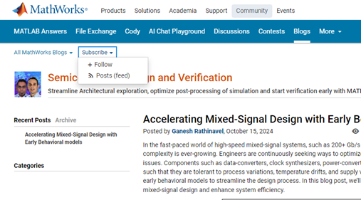
Don’t miss the first post: Accelerating Mixed-Signal Design with Early Behavioral Models, where they explore how early behavioral modeling can accelerate mixed-signal design and enhance system efficiency.
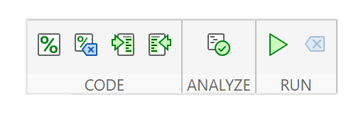
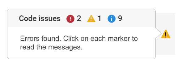
We are happy to announce the addition of a new code analyzing feature to the AI Chat Playground. This new feature allows you to identify issues with your code making it easier to troubleshoot.
How does it work?
Just click the ANALYZE button in the toolbar of the code editor. Your code is sent to MATLAB running on a server which returns any warnings or errors, each of which are associated to a line of code on the right side of the editor window. Hover over each line marker to view the message.
Give it a try and share your feedback here. We will be adding this new capability to other community areas in the future so your feedback is appreciated.
Thank you,
David
There are so many incredible entries created in week 1. Now, it’s time to announce the weekly winners in various categories!
Nature & Space:
Seamless Loop:
Abstract:
Remix of previous Mini Hack entries:
Early Discovery
Holiday:
Congratulations to all winners! Each of you won your choice of a T-shirt, a hat, or a coffee mug. We will contact you after the contest ends.
In week 2, we’d love to see and award more entries in the ‘Seamless Loop’ category. We can't wait to see your creativity shine!
Tips for Week 2:
1.Use AI for assistance
The code from the Mini Hack entries can be challenging, even for experienced MATLAB users. Utilize AI tools for MATLAB to help you understand the code and modify the code. Here is an example of a remix assisted by AI. @Hans Scharler used MATLAB GPT to get an explanation of the code and then prompted it to ‘change the background to a starry night with the moon.’
2. Share your thoughts
Share your tips & tricks, experience of using AI, or learnings with the community. Post your knowledge in the Discussions' general channel (be sure to add the tag 'contest2024') to earn opportunities to win the coveted MATLAB Shorts.
3. Ensure Thumbnails Are Displayed:
You might have noticed that some entries on the leaderboard lack a thumbnail image. To fix this, ensure you include ‘drawframe(1)’ in your code.
Over the past week, we have seen many creative and compelling short movies! Now, let the voting begin! Cast your votes for the short movies you love. Authors, share your creations with friends, classmates, and colleagues. Let's showcase the beauty of mathematics to the world!
We know that one of the key goals for joining the Mini Hack contest is to LEARN! To celebrate knowledge sharing, we have special prizes—limited-edition MATLAB Shorts—up for grabs!
These exclusive prizes can only be earned through the MATLAB Shorts Mini Hack contest. Interested? Share your knowledge in the Discussions' general channel (be sure to add the tag 'contest2024') to earn opportunities to win the coveted MATLAB Shorts. You can share various types of content, such as tips and tricks for creating animations, background stories of your entry, or learnings you've gained from the contest. We will select different types of winners each week.

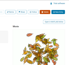
We also have an exciting feature announcement: you can now experiment with code in MATLAB Online. Simply click the 'Open in MATLAB Online' button above the movie preview section. Even better! ‘Open in MATLAB Online’ is also available in previous Mini Hack contests!
We look forward to seeing more amazing short movies in Week 2!
function drawframe(f)
% Create a figure
figure;
hold on;
axis equal;
axis off;
% Draw the roads
rectangle('Position', [0, 0, 2, 30], 'FaceColor', [0.5 0.5 0.5]); % Left road
rectangle('Position', [2, 0, 2, 30], 'FaceColor', [0.5 0.5 0.5]); % Right road
% Draw the traffic light
trafficLightPole = rectangle('Position', [-1, 20, 1, 0.2], 'FaceColor', 'black'); % Pole
redLight = rectangle('Position', [0, 20, 0.5, 1], 'FaceColor', 'red'); % Red light
yellowLight = rectangle('Position', [0.5, 20, 0.5, 1], 'FaceColor', 'black'); % Yellow light
greenLight = rectangle('Position', [1, 20, 0.5, 1], 'FaceColor', 'black'); % Green light
carBody = rectangle('Position', [2.5, 2, 1, 4], 'Curvature', 0.2, 'FaceColor', 'red'); % Body
leftWheel = rectangle('Position', [2.5, 3.0, 0.2, 0.2], 'Curvature', [1, 1], 'FaceColor', 'black'); % Left wheel
rightWheel = rectangle('Position', [3.3, 3.0, 0.2, 0.2], 'Curvature', [1, 1], 'FaceColor', 'black'); % Right wheel
leftFrontWheel = rectangle('Position', [2.5, 5.0, 0.2, 0.2], 'Curvature', [1, 1], 'FaceColor', 'black'); % Left wheel
rightFrontWheel = rectangle('Position', [3.3, 5.0, 0.2, 0.2], 'Curvature', [1, 1], 'FaceColor', 'black'); % Right wheel
% Set limits
xlim([-1, 8]);
ylim([-1, 35]);
% Animation parameters
carSpeed = 0.5; % Speed of the car
carPosition = 2; % Initial car position
stopPosition = 15; % Position to stop at the traffic light
isStopped = false; % Car is not stopped initially
%Animation loop
for t = 1:100
% Update traffic light: Red for 40 frames, yellow for 10 frames Green for 40 frames
if t <= 40
% Red light on, yellow and green off
set(redLight, 'FaceColor', 'red');
set(yellowLight, 'FaceColor', 'black');
set(greenLight, 'FaceColor', 'black');
elseif t > 40 && t <= 50
% Change to green light
set(redLight, 'FaceColor', 'black');
set(yellowLight, 'FaceColor', 'yellow');
set(greenLight, 'FaceColor', 'black');
else
% Back to red light
set(redLight, 'FaceColor', 'black');
set(yellowLight, 'FaceColor', 'black');
set(greenLight, 'FaceColor', 'green');
isStopped = false; % Allow car to move
end
%Move the car
if ~isStopped
carPosition = carPosition + carSpeed; % Move forward
if carPosition < stopPosition
%do nothing
else
isStopped = true;
end
else
% Gradually stop the car when red
if carPosition > stopPosition
carPosition = carPosition + carSpeed*(1-t/50); % Move backward until it reaches the stop position
end
end
if carPosition >= 25
carPosition = 25;
end
% Update car position
% set(carBody, 'Position', [carPosition, 2, 1, 0.5]);
set(carBody, 'Position', [2.5, carPosition, 1, 4]);
%set(carWindow, 'Position', [carPosition + 0.2, 2.4, 0.6, 0.2]);
%set(leftWheel, 'Position', [carPosition, 1.5, 0.2, 0.2]);
set(leftWheel, 'Position', [2.5, carPosition+1, 0.2, 0.2]);
% set(rightWheel, 'Position', [carPosition + 0.8, 1.5, 0.2, 0.2]);
set(rightWheel, 'Position', [3.3, carPosition+1, 0.2, 0.2]);
set(leftFrontWheel, 'Position', [2.5, carPosition+3, 0.2, 0.2]);
set(rightFrontWheel, 'Position', [3.3, carPosition+3, 0.2, 0.2]);
% Pause to control animation speed
pause(0.01);
end
hold off;
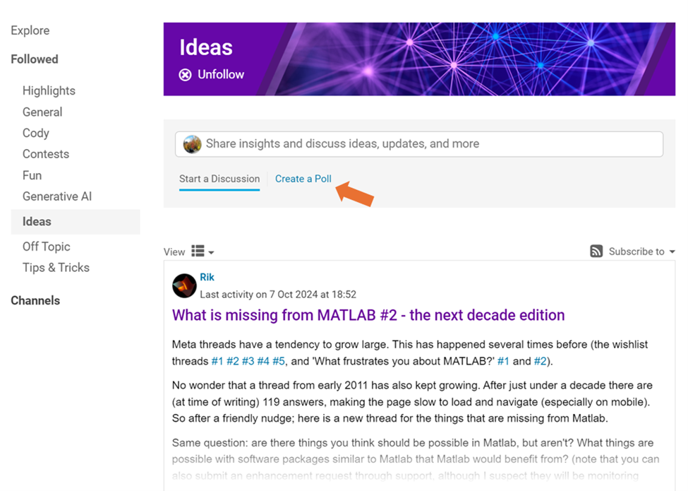
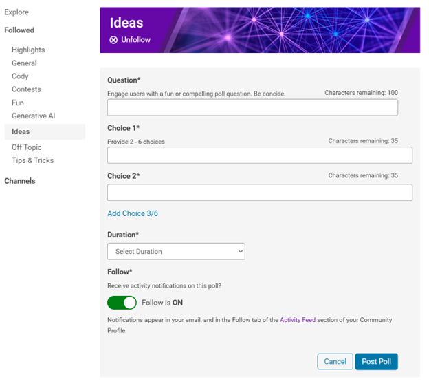
We are thrilled to announce that every community member now has the ability to create a poll in Discussions, allowing you to gather votes and opinions from the community.
How to create a poll:
You can find the ‘Create a Poll’ link just below the text box (see screenshot below). Please note that the default type of content is a ‘Discussion’. To start a poll, simply click the link.
Creating a poll is straightforward. You can add up to 6 choices for your poll and set the duration from 1 to 6 weeks.
Where to find the poll
Polls created by community members will appear only in the channel where they are created and the landing page of Discussions area. Discussions moderators have the privilege to feature/broadcast the poll across Answers, File Exchange, and Cody.
Thoughts?
We can’t wait to see what interesting polls our community will create. Meanwhile, if you have any questions or suggestions, feel free to leave a comment.
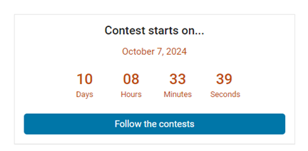
We're excited to announce that the 2024 Community Contest—MATLAB Shorts Mini Hack starts today! The contest will run for 5 weeks, from Oct. 7th to Nov. 10th.
What creative short movies will you create? Let the party begin, and we look forward to seeing you all in the contest!
If you are interested in AI, Autonomous Systems and Robotics, and the future of engineering, don't miss out on MATLAB EXPO 2024 and register now.
You will have the opportunity to connect with engineers, scientists, educators, and researchers, and new ideas.
Featured Sessions:
- From Embedded to Empowered: The Rise of Software-Defined Products - María Elena Gavilán Alfonso, MathWorks
- The Empathetic Engineers of Tomorrow - Dr. Darryll Pines, University of Maryland
- A Model-Based Design Journey from Aerospace to an Artificial Pancreas System - Louis Lintereur, Medtronic Diabetes
Featured Topics:
- AI
- Autonomous Systems and Robotics
- Electrification
- Algorithm Development and Data Analysis
- Modeling, Simulation, Verification, Validation, and Implementation
- Wireless Communications
- Cloud, Software Factories, and DevOps
- Preparing Future Engineers and Scientists

We are thrilled to announce the redesign of the Discussions leaf page, with a new user-focused right-hand column!

Why Are We Doing This?
- Address Readers’ Needs:
Previously, the right-hand column displayed related content, but feedback from our community indicated that this wasn't meeting your needs. Many of you expressed a desire to read more posts from the same author but found it challenging to locate them.
With the new design, readers can easily learn more about the author, explore their other posts, and follow them to receive notifications on new content.
- Enhance Authors’ Experience:
Since the launch of the Discussions area earlier this year, we've seen an influx of community members sharing insightful technical articles, use cases, and ideas. The new design aims to help you grow your followers and organize your content more effectively by editing tags. We highly encourage you to use the Discussions area as your community blogging platform.
We hope you enjoy the new design of the right-hand column. Please feel free to share your thoughts and experiences by leaving a comment below.
Dear contest participants,
The 2024 Community Contest—MATLAB Shorts Mini Hack—is just one week away! Last year, we challenged you to create a 48-frame, 2-second animation. This year, we're doubling the fun by increasing the frame count to 96 and adding audio support. Your mission? Create a short movie!
As always, whether you are a seasoned MATLAB user or just a beginner, you can participate in the contest and have opportunities to win amazing prizes.

Timeframe:
- The contest will run for 5 weeks, from Oct. 7th to Nov. 10th, Eastern Time.
General Rules:
- The first week is dedicated to entry creation, and the fifth week is reserved for voting only.
- Create a 96-frame, 4-second animation and add audio. We will loop it 3 times to create a 12-second short movie for you.
- The character limit remains at 2,000 characters.
Prizes
- You will have opportunities to win compelling prizes, including Amazon gift cards, MathWorks T-shirts, and virtual badges. We will give out both weekly prizes and grand prizes.
Warm-up!
With one week left before the contest begins, we recommend you warm up by reading a fantastic article: Walkthrough: making Little Nemo's airship in MATLAB by @Tim. The article shares both technical insights and the challenges encountered along the way.
The MATLAB Central Community Team
We are excited to invite you to join our 2024 community contest – MATLAB Shorts Mini Hack! Last year, we challenged you to create a 48-frame animation. In 2024, we are increasing the frame count to 96 and supporting audio. Your mission? Create a short movie!
Whether you are a seasoned MATLAB user or just a beginner, you can participate in the contest and have opportunities to win amazing prizes. Be sure to check out our Blog post for more details on the Community Contests.
Timeframe
This contest runs for 5 weeks, from Oct. 7th to Nov. 10th.
How to Participate
- Create a new short movie or remix an existing one with up to 2,000 characters of code.
- Vote or comment on the short movies you love!
Prizes
You will have opportunities to win compelling prizes, including Amazon gift cards, MathWorks T-shirts, and virtual badges. We will give out both weekly prizes and grand prizes.
Stay Informed
Make sure to follow the contest to get important announcements and your prize updates.