主要内容
Results for
Welcome to the launch of our new blog area, Semiconductor Design and Verification! The mission is to empower engineers and designers in the semiconductor industry by streamlining architectural exploration, optimizing the post-processing of simulations, and enabling early verification with MATLAB and Simulink.
Meet Our Authors
We are thrilled to have two esteemed authors:
@Ganesh Rathinavel and @Cristian Macario Macario have both made significant contributions to the advancement of Analog/Mixed-Signal design and the broader communications, electronics, and semiconductor industries. With impressive engineering backgrounds and extensive experience at leading companies such as IMEC, STMicroelectronics, NXP Semiconductors, LSI Corporation, and ARM, they bring a wealth of knowledge and expertise to our blog. Their work is focused on enhancing MathWorks' tools to better align with industry needs.
What to Expect
The blog will cover a wide range of topics aimed at professionals in the semiconductor field, providing insights and strategies to enhance your design and verification processes. Whether you're looking to streamline your current workflows or explore cutting-edge methodologies, our blog is your go-to resource.
Call to Action
We invite all professionals and enthusiasts in the semiconductor industry to follow our blog posts. Stay updated with the latest trends and insights by subscribing to our blog.
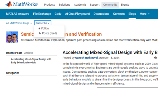
Don’t miss the first post: Accelerating Mixed-Signal Design with Early Behavioral Models, where they explore how early behavioral modeling can accelerate mixed-signal design and enhance system efficiency.
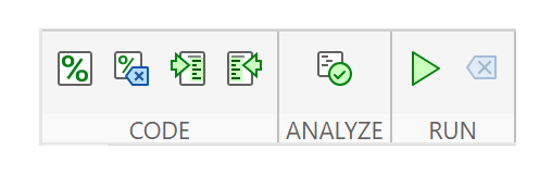
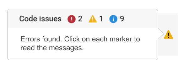
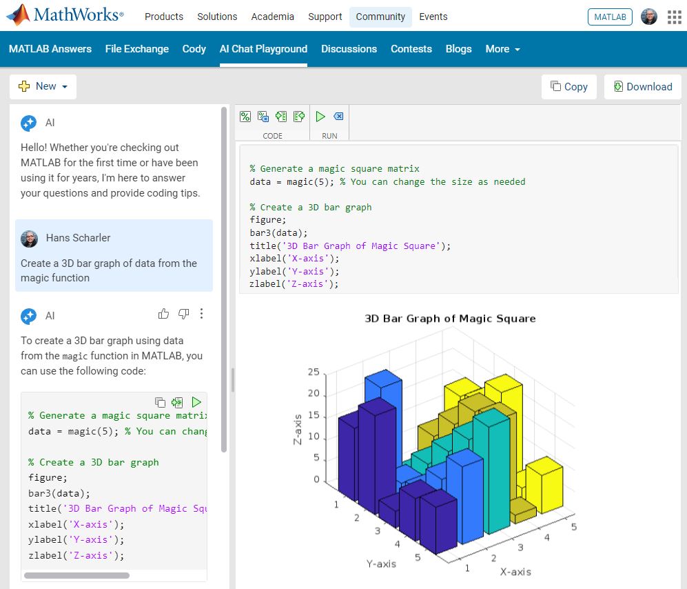
We are happy to announce the addition of a new code analyzing feature to the AI Chat Playground. This new feature allows you to identify issues with your code making it easier to troubleshoot.
How does it work?
Just click the ANALYZE button in the toolbar of the code editor. Your code is sent to MATLAB running on a server which returns any warnings or errors, each of which are associated to a line of code on the right side of the editor window. Hover over each line marker to view the message.
Give it a try and share your feedback here. We will be adding this new capability to other community areas in the future so your feedback is appreciated.
Thank you,
David
There are so many incredible entries created in week 1. Now, it’s time to announce the weekly winners in various categories!
Nature & Space:
Seamless Loop:
Abstract:
Remix of previous Mini Hack entries:
Early Discovery
Holiday:
Congratulations to all winners! Each of you won your choice of a T-shirt, a hat, or a coffee mug. We will contact you after the contest ends.
In week 2, we’d love to see and award more entries in the ‘Seamless Loop’ category. We can't wait to see your creativity shine!
Tips for Week 2:
1.Use AI for assistance
The code from the Mini Hack entries can be challenging, even for experienced MATLAB users. Utilize AI tools for MATLAB to help you understand the code and modify the code. Here is an example of a remix assisted by AI. @Hans Scharler used MATLAB GPT to get an explanation of the code and then prompted it to ‘change the background to a starry night with the moon.’
2. Share your thoughts
Share your tips & tricks, experience of using AI, or learnings with the community. Post your knowledge in the Discussions' general channel (be sure to add the tag 'contest2024') to earn opportunities to win the coveted MATLAB Shorts.
3. Ensure Thumbnails Are Displayed:
You might have noticed that some entries on the leaderboard lack a thumbnail image. To fix this, ensure you include ‘drawframe(1)’ in your code.
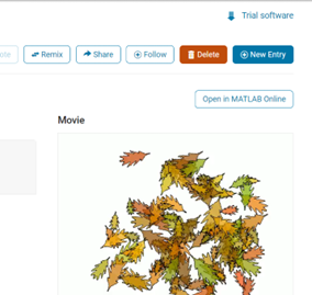
Over the past week, we have seen many creative and compelling short movies! Now, let the voting begin! Cast your votes for the short movies you love. Authors, share your creations with friends, classmates, and colleagues. Let's showcase the beauty of mathematics to the world!
We know that one of the key goals for joining the Mini Hack contest is to LEARN! To celebrate knowledge sharing, we have special prizes—limited-edition MATLAB Shorts—up for grabs!
These exclusive prizes can only be earned through the MATLAB Shorts Mini Hack contest. Interested? Share your knowledge in the Discussions' general channel (be sure to add the tag 'contest2024') to earn opportunities to win the coveted MATLAB Shorts. You can share various types of content, such as tips and tricks for creating animations, background stories of your entry, or learnings you've gained from the contest. We will select different types of winners each week.

We also have an exciting feature announcement: you can now experiment with code in MATLAB Online. Simply click the 'Open in MATLAB Online' button above the movie preview section. Even better! ‘Open in MATLAB Online’ is also available in previous Mini Hack contests!
We look forward to seeing more amazing short movies in Week 2!
function drawframe(f)
% Create a figure
figure;
hold on;
axis equal;
axis off;
% Draw the roads
rectangle('Position', [0, 0, 2, 30], 'FaceColor', [0.5 0.5 0.5]); % Left road
rectangle('Position', [2, 0, 2, 30], 'FaceColor', [0.5 0.5 0.5]); % Right road
% Draw the traffic light
trafficLightPole = rectangle('Position', [-1, 20, 1, 0.2], 'FaceColor', 'black'); % Pole
redLight = rectangle('Position', [0, 20, 0.5, 1], 'FaceColor', 'red'); % Red light
yellowLight = rectangle('Position', [0.5, 20, 0.5, 1], 'FaceColor', 'black'); % Yellow light
greenLight = rectangle('Position', [1, 20, 0.5, 1], 'FaceColor', 'black'); % Green light
carBody = rectangle('Position', [2.5, 2, 1, 4], 'Curvature', 0.2, 'FaceColor', 'red'); % Body
leftWheel = rectangle('Position', [2.5, 3.0, 0.2, 0.2], 'Curvature', [1, 1], 'FaceColor', 'black'); % Left wheel
rightWheel = rectangle('Position', [3.3, 3.0, 0.2, 0.2], 'Curvature', [1, 1], 'FaceColor', 'black'); % Right wheel
leftFrontWheel = rectangle('Position', [2.5, 5.0, 0.2, 0.2], 'Curvature', [1, 1], 'FaceColor', 'black'); % Left wheel
rightFrontWheel = rectangle('Position', [3.3, 5.0, 0.2, 0.2], 'Curvature', [1, 1], 'FaceColor', 'black'); % Right wheel
% Set limits
xlim([-1, 8]);
ylim([-1, 35]);
% Animation parameters
carSpeed = 0.5; % Speed of the car
carPosition = 2; % Initial car position
stopPosition = 15; % Position to stop at the traffic light
isStopped = false; % Car is not stopped initially
%Animation loop
for t = 1:100
% Update traffic light: Red for 40 frames, yellow for 10 frames Green for 40 frames
if t <= 40
% Red light on, yellow and green off
set(redLight, 'FaceColor', 'red');
set(yellowLight, 'FaceColor', 'black');
set(greenLight, 'FaceColor', 'black');
elseif t > 40 && t <= 50
% Change to green light
set(redLight, 'FaceColor', 'black');
set(yellowLight, 'FaceColor', 'yellow');
set(greenLight, 'FaceColor', 'black');
else
% Back to red light
set(redLight, 'FaceColor', 'black');
set(yellowLight, 'FaceColor', 'black');
set(greenLight, 'FaceColor', 'green');
isStopped = false; % Allow car to move
end
%Move the car
if ~isStopped
carPosition = carPosition + carSpeed; % Move forward
if carPosition < stopPosition
%do nothing
else
isStopped = true;
end
else
% Gradually stop the car when red
if carPosition > stopPosition
carPosition = carPosition + carSpeed*(1-t/50); % Move backward until it reaches the stop position
end
end
if carPosition >= 25
carPosition = 25;
end
% Update car position
% set(carBody, 'Position', [carPosition, 2, 1, 0.5]);
set(carBody, 'Position', [2.5, carPosition, 1, 4]);
%set(carWindow, 'Position', [carPosition + 0.2, 2.4, 0.6, 0.2]);
%set(leftWheel, 'Position', [carPosition, 1.5, 0.2, 0.2]);
set(leftWheel, 'Position', [2.5, carPosition+1, 0.2, 0.2]);
% set(rightWheel, 'Position', [carPosition + 0.8, 1.5, 0.2, 0.2]);
set(rightWheel, 'Position', [3.3, carPosition+1, 0.2, 0.2]);
set(leftFrontWheel, 'Position', [2.5, carPosition+3, 0.2, 0.2]);
set(rightFrontWheel, 'Position', [3.3, carPosition+3, 0.2, 0.2]);
% Pause to control animation speed
pause(0.01);
end
hold off;
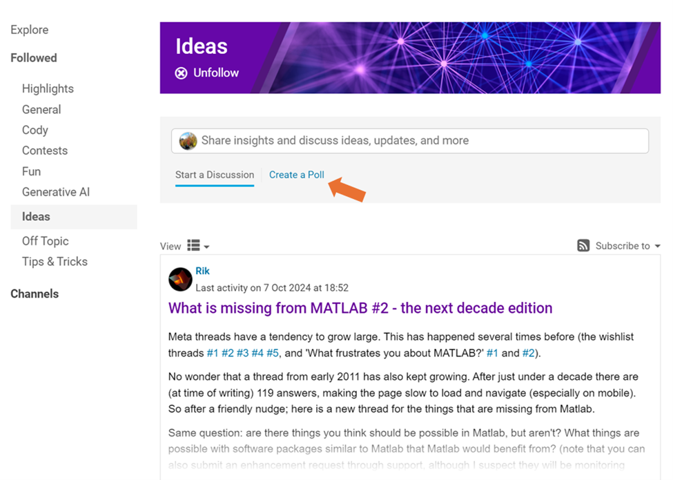
We are thrilled to announce that every community member now has the ability to create a poll in Discussions, allowing you to gather votes and opinions from the community.
How to create a poll:
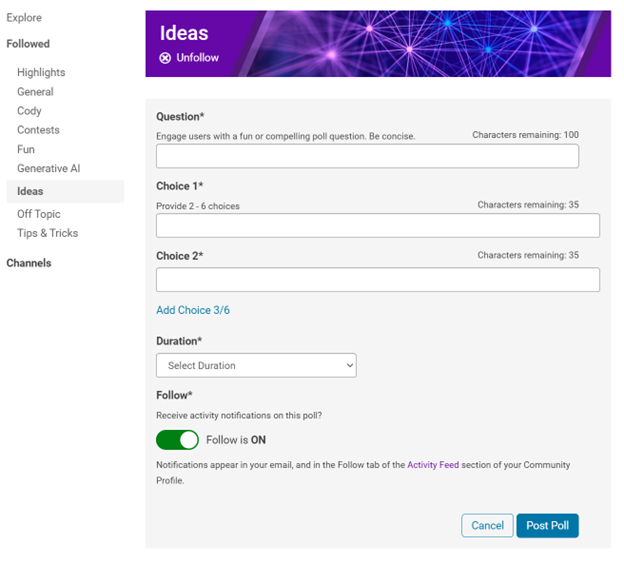
You can find the ‘Create a Poll’ link just below the text box (see screenshot below). Please note that the default type of content is a ‘Discussion’. To start a poll, simply click the link.
Creating a poll is straightforward. You can add up to 6 choices for your poll and set the duration from 1 to 6 weeks.
Where to find the poll
Polls created by community members will appear only in the channel where they are created and the landing page of Discussions area. Discussions moderators have the privilege to feature/broadcast the poll across Answers, File Exchange, and Cody.
Thoughts?
We can’t wait to see what interesting polls our community will create. Meanwhile, if you have any questions or suggestions, feel free to leave a comment.
hello i found the following tools helpful to write matlab programs. copilot.microsoft.com chatgpt.com/gpts gemini.google.com and ai.meta.com. thanks a lot and best wishes.
We're excited to announce that the 2024 Community Contest—MATLAB Shorts Mini Hack starts today! The contest will run for 5 weeks, from Oct. 7th to Nov. 10th.
What creative short movies will you create? Let the party begin, and we look forward to seeing you all in the contest!
If I go to a paint store, I can get foldout color charts/swatches for every brand of paint. I can make a selection and it will tell me the exact proportions of each of base color to add to a can of white paint. There doesn't seem to be any equivalent in MATLAB. The common word "swatch" doesn't even exist in the documentation. (?) One thinks pcolor() would be the way to go about this, but pcolor documentation is the most abstruse in all of the documentation. Thanks 1e+06 !
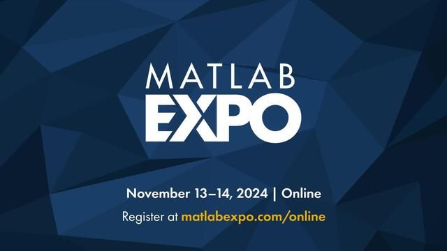
If you are interested in AI, Autonomous Systems and Robotics, and the future of engineering, don't miss out on MATLAB EXPO 2024 and register now.
You will have the opportunity to connect with engineers, scientists, educators, and researchers, and new ideas.
Featured Sessions:
- From Embedded to Empowered: The Rise of Software-Defined Products - María Elena Gavilán Alfonso, MathWorks
- The Empathetic Engineers of Tomorrow - Dr. Darryll Pines, University of Maryland
- A Model-Based Design Journey from Aerospace to an Artificial Pancreas System - Louis Lintereur, Medtronic Diabetes
Featured Topics:
- AI
- Autonomous Systems and Robotics
- Electrification
- Algorithm Development and Data Analysis
- Modeling, Simulation, Verification, Validation, and Implementation
- Wireless Communications
- Cloud, Software Factories, and DevOps
- Preparing Future Engineers and Scientists
We are thrilled to announce the redesign of the Discussions leaf page, with a new user-focused right-hand column!
Why Are We Doing This?
- Address Readers’ Needs:
Previously, the right-hand column displayed related content, but feedback from our community indicated that this wasn't meeting your needs. Many of you expressed a desire to read more posts from the same author but found it challenging to locate them.
With the new design, readers can easily learn more about the author, explore their other posts, and follow them to receive notifications on new content.
- Enhance Authors’ Experience:
Since the launch of the Discussions area earlier this year, we've seen an influx of community members sharing insightful technical articles, use cases, and ideas. The new design aims to help you grow your followers and organize your content more effectively by editing tags. We highly encourage you to use the Discussions area as your community blogging platform.
We hope you enjoy the new design of the right-hand column. Please feel free to share your thoughts and experiences by leaving a comment below.
As pointed out in Doxygen comments in code generated with Simulink Embedded Coder - MATLAB Answers - MATLAB Central (mathworks.com), it would be nice that Embedded Coder has an option to generate Doxygen-style comments for signals of buses, i.e.:
/** @brief <Signal desciption here> **/
This would allow static analysis tools to parse the comments. Please add that feature!
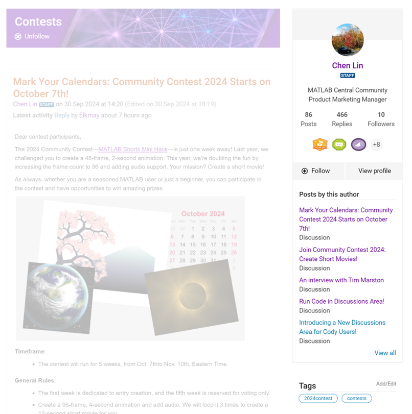
Dear contest participants,
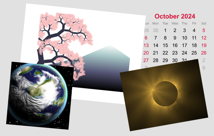
The 2024 Community Contest—MATLAB Shorts Mini Hack—is just one week away! Last year, we challenged you to create a 48-frame, 2-second animation. This year, we're doubling the fun by increasing the frame count to 96 and adding audio support. Your mission? Create a short movie!
As always, whether you are a seasoned MATLAB user or just a beginner, you can participate in the contest and have opportunities to win amazing prizes.
Timeframe:
- The contest will run for 5 weeks, from Oct. 7th to Nov. 10th, Eastern Time.
General Rules:
- The first week is dedicated to entry creation, and the fifth week is reserved for voting only.
- Create a 96-frame, 4-second animation and add audio. We will loop it 3 times to create a 12-second short movie for you.
- The character limit remains at 2,000 characters.
Prizes
- You will have opportunities to win compelling prizes, including Amazon gift cards, MathWorks T-shirts, and virtual badges. We will give out both weekly prizes and grand prizes.
Warm-up!
With one week left before the contest begins, we recommend you warm up by reading a fantastic article: Walkthrough: making Little Nemo's airship in MATLAB by @Tim. The article shares both technical insights and the challenges encountered along the way.
The MATLAB Central Community Team
We are excited to invite you to join our 2024 community contest – MATLAB Shorts Mini Hack! Last year, we challenged you to create a 48-frame animation. In 2024, we are increasing the frame count to 96 and supporting audio. Your mission? Create a short movie!
Whether you are a seasoned MATLAB user or just a beginner, you can participate in the contest and have opportunities to win amazing prizes. Be sure to check out our Blog post for more details on the Community Contests.
Timeframe
This contest runs for 5 weeks, from Oct. 7th to Nov. 10th.
How to Participate
- Create a new short movie or remix an existing one with up to 2,000 characters of code.
- Vote or comment on the short movies you love!
Prizes
You will have opportunities to win compelling prizes, including Amazon gift cards, MathWorks T-shirts, and virtual badges. We will give out both weekly prizes and grand prizes.
Stay Informed
Make sure to follow the contest to get important announcements and your prize updates.
The AI Chat Playground at MATLAB Central has two new upgrades: OpenAI GPT-4o mini and MATLAB R2024b!
GPT-4o mini is a new language model from OpenAI and brings general knowledge up to October 2023. GPT-4o mini surpasses GPT-3.5 Turbo and other small models on academic benchmarks across both textual intelligence and reasoning. Our goal is to keep improving the output of the AI Chat Playground. This upgrade is available now: https://www.mathworks.com/matlabcentral/playground/
One more thing... we also updated the system to the latest release of MATLAB. This is R2024b and comes with hundreds of updates and new plot types to explore.Check out Mike Croucher's blog post about the latest version of MATLAB: https://blogs.mathworks.com/matlab/2024/09/13/the-latest-version-of-matlab-r2024b-has-just-been-released/
We are looking forward to your feedback on the updates to the AI Chat Playground. Let us know what you think and how you use this community app.
Always!
29%
It depends
14%
Never!
21%
I didn't know that was possible
36%
1810 个投票
In the spirit of warming up for this year's minihack contest, I'm uploading a walkthrough for how to design an airship using pure Matlab script. This is commented and uncondensed; half of the challenge for the minihacks is how minimize characters. But, maybe it will give people some ideas.
The actual airship design is from one of my favorite original NES games that I played when I was a kid - Little Nemo: The Dream Master. The design comes from the intro of the game when Nemo sees the Slumberland airship leave for Slumberland:
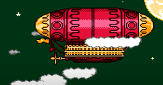
(Snip from a frame of the opening scene in Capcom's game Little Nemo: The Dream Master, showing the Slumberland airship).
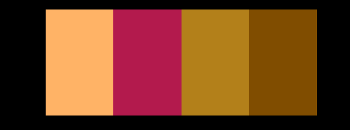
I spent hours playing this game with my two sisters, when we were little. It's fun and tough, but the graphics sparked the imagination. On to the code walkthrough, beginning with the color palette: these four colors are the only colors used for the airship:
c1=cat(3,1,.7,.4); % Cream color
c2=cat(3,.7,.1,.3); % Magenta
c3=cat(3,0.7,.5,.1); % Gold
c4=cat(3,.5,.3,0); % bronze
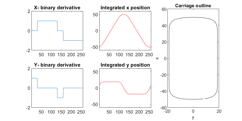
We start with the airship carriage body. We want something rectangular but smoothed on the corners. To do this we are going to start with the separate derivatives of the x and y components, which can be expressed using separate blocks of only three levels: [1, 0, -1]. You could integrate to create a rectangle, but if we smooth the derivatives prior to integrating we will get rounded edges. This is done in the following code:
% Binary components for x & y vectors
z=zeros(1,30);
o=ones(1,100);
% X and y vectors
x=[z,o,z,-o];
y=[1+z,1-o,z-1,1-o];
% Smoother function (fourier / circular)
s=@(x)ifft(fft(x).*conj(fft(hann(45)'/22,260)));
% Integrator function with replication and smoothing to form mesh matrices
u=@(x)repmat(cumsum(s(x)),[30,1]);
% Construct x and y components of carriage with offsets
x3=u(x)-49.35;
y3=u(y)+6.35;
y3 = y3*1.25; % Make it a little fatter
% Add a z-component to make the full set of matrices for creating a 3D
% surface:
z3=linspace(0,1,30)'.*ones(1,260)*30;
z3(14,:)=z3(15,:); % These two lines are for adding platforms
z3(2,:)=z3(3,:); % to the carriage, later.
Plotting x, y, and the top row of the smoothed, integrated, and replicated matrices x3 and y3 gives the following:
We now have the x and y components for a 3D mesh of the carriage, let's make it more interesting by adding a color scheme including doors, and texture for the trim around the doors. Let's also add platforms beneath the doors for passengers to walk on.
Starting with the color values, let's make doors by convolving points in a color-matrix by a door shaped function.
m=0*z3; % Image matrix that will be overlayed on carriage surface
m(7,10:12:end)=1; % Door locations (lower deck)
m(21,10:12:end)=1; % Door locations (upper deck)
drs = ones(9, 5); % Door shape
m=1-conv2(m,ones(9,5),'same'); % Applying
To add the trim, we will convolve matrix "m" (the color matrix) with a square function, and look for values that lie between the extrema. We will use this to create a displacement function that bumps out the -x, and -y values of the carriage surface in intermediary polar coordinate format.
rm=conv2(m,ones(5)/25,'same'); % Smoothing the door function
rm(~m)=0; % Preserving only the region around the doors
rds=0*m; % Radial displacement function
rds(rm<1&rm>0)=1; % Preserving region around doors
rds(m==0)=0;
rds(13:14,:)=6; % Adding walkways
rds(1:2,:)=6;
% Apply radial displacement function
[th,rd]=cart2pol(x3,y3);
[x3T,y3T]=pol2cart(th,(rd+rds)*.89);
If we plot the color function (m) and radial displacement function (rds) we get the following:
In the upper plot you can see the doors, and in the bottom map you can see the walk way and door trim.
Next, we are going to add some flags draped from the bottom and top of the carriage. We are going to recycle the values in "z3" to do this, by multiplying that matrix with the absolute value of a sine-wave, squished a bit with the soft-clip erf() function.
We add a keel to the airship carriage using a canonical sphere turned on its side, again using the soft-clip erf() function to make it roughly rectangular in x and y, and multiplying with a vector that is half nan's to make the top half transparent.
At this point, since we are beginning the plotting of the ship, we also need to create our hgtransform objects. These allow us to move all of the components of the airship in unison, and also link objects with pivot points to the airship, such as the propeller.
% Now we need some flags extending around the top and bottom of the
% carriage. We can do this my multiplying the height function (z3) with the
% absolute value of a sine-wave, rounded with a compression function
% (erf() in this case);
g=-z3.*erf(abs(sin(linspace(0,40*pi,260))))/4; % Flags
% Also going to add a slight taper to the carriage... gives it a nice look
tp=linspace(1.05,1,30)';
% Finally, plotting. Plot the carriage with the color-map for the doors in
% the cream color, than the flags in magenta. Attach them both to transform
% objects for movement.
% Set up transform objects. 2 moving parts:
% 1) The airship itself and all sub-components
% 2) The propellor, which attaches to the airship and spins on its axis.
hold on;
P=hgtransform('Parent',gca); % Ship
S=hgtransform('Parent',P); % Prop
surf(x3T.*tp,y3T,z3,c1.*m,'Parent',P);
surf(x3,y3,g,c2.*rd./rd, 'Parent', P);
surf(x3,y3,g+31,c2.*rd./rd, 'Parent', P);
axis equal
% Now add the keel of the airship. Will use a canonical sphere and the
% erf() compression function to square off.
[x,y,z]=sphere(99);
mk=round(linspace(-1,1).^2+.3); % This function makes the top half of the sphere nan's for transparency.
surf(50*erf(1.4*z),15*erf(1.4*y),13*x.*mk./mk-1,.5*c2.*z./z, 'Parent', P);
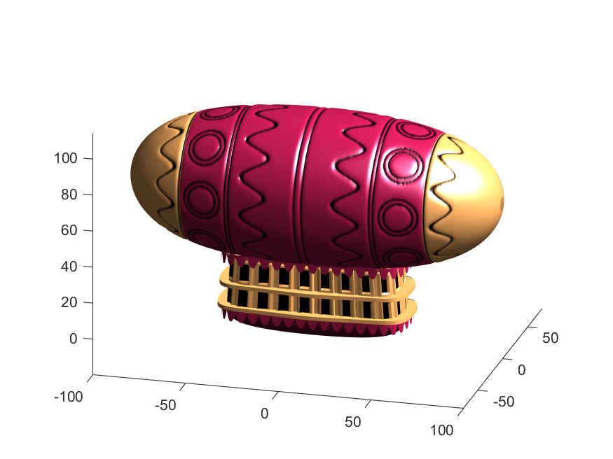
% The carriage is done. Now we can make the blimp above it.
We haven't adjusted the shading of the image yet, but you can see the design features that have been created:
Next, we start working on the blimp. This is going to use a few more vertices & faces. We are going to use a tapered cylinder for this part, and will start by making the overlaid image, which will have 2 colors plus radial rings, circles, and squiggles for ornamentation.
M=525; % Blimp (matrix dimensions)
N=700;
% Assign the blimp the cream and magenta colors
t=122; % Transition point
b=ones(M,N,3); % Blimp color map template
bc=b.*c1; % Blimp color map
bc(:,t+1:end-t,:)=b(:,t+1:end-t,:).*c2;
% Add axial rings around blimp
l=[.17,.3,.31,.49];
l=round([l,1-fliplr(l)]*N); % Mirroring
lnw=ones(1,N); % Mask
lnw(l)=0;
lnw=rescale(conv(lnw,hann(7)','same'));
bc=bc.*lnw;
% Now add squiggles. We're going to do this by making an even function in
% the x-dimension (N, 725) added with a sinusoidal oscillation in the
% y-dimension (M, 500), then thresholding.
r=sin(linspace(0, 2*pi, M)*10)'+(linspace(-1, 1, N).^6-.18)*15;
q=abs(r)>.15;
r=sin(linspace(0, 2*pi, M)*12)'+(abs(linspace(-1, 1, N))-.25)*15;
q=q.*(abs(r)>.15);
% Now add the circles on the blimp. These will be spaced evenly in the
% polar angle dimension around the axis. We will have 9. To make the
% circles, we will create a cone function with a peak at the center of the
% circle, and use thresholding to create a ring of appropriate radius.
hs=[1,.75,.5,.25,0,-.25,-.5,-.75,-1]; % Axial spacing of rings
% Cone generation and ring loop
xy= @(h,s)meshgrid(linspace(-1, 1, N)+s*.53,(linspace(-1, 1, M)+h)*1.15);
w=@(x,y)sqrt(x.^2+y.^2);
for n=1:9
h=hs(n);
[xx,yy]=xy(h,-1);
r1=w(xx,yy);
[xx,yy]=xy(h,1);
r2=w(xx,yy);
b=@(x,y)abs(y-x)>.005;
q=q.*b(.1,r1).*b(.075,r1).*b(.1,r2).*b(.075,r2);
end
The figures below show the color scheme and mask used to apply the squiggles and circles generated in the code above:
Finally, for the colormap we are going to smooth the binary mask to avoid hard transitions, and use it to to add a "puffy" texture to the blimp shape. This will be done by diffusing the mask iteratively in a loop with a non-linear min() operator.
% 2D convolution function
ff=@(x)circshift(ifft2(fft2(x).*conj(fft2(hann(7)*hann(7)'/9,M,N))),[3,3]);
q=ff(q); % Smooth our mask function
hh=rgb2hsv(q.*bc); % Convert to hsv: we are going to use the value
% component for radial displacement offsets of the
% 3D blimp structure.
rd=hh(:,:,3); % Value component
for n=1:10
rd=min(rd,ff(rd)); % Diffusing the value component for a puffy look
end
rd=(rd+35)/36; % Make displacements effects small
% Now make 3D blimp manifold using "cylinder" canonical shape
[x,y,z]=cylinder(erf(sin(linspace(0,pi,N)).^.5)/4,M-1); % First argument is the blimp taper
[t,r]=cart2pol(x, y);
[x2,y2]=pol2cart(t, r.*rd'); % Applying radial displacment from mask
s=200;
% Plotting the blimp
surf(z'*s-s/2, y2'*s, x2'*s+s/3.9+15, q.*bc,'Parent',P);
Notice that the parent of the blimp surface plot is the same as the carriage (e.g. hgtransform object "P"). Plotting at this point using flat shading and adding some lighting gives the image below:
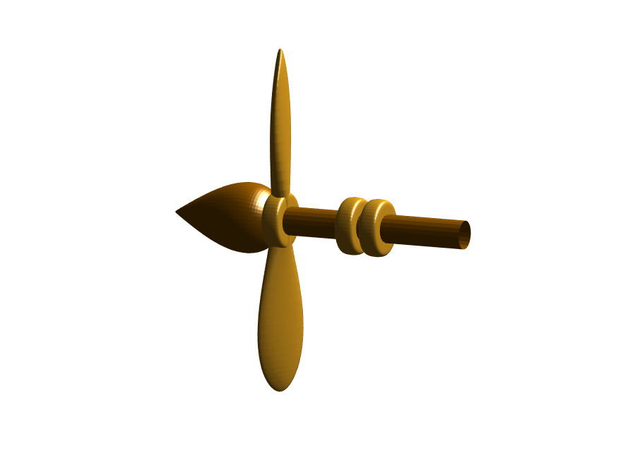
Next, we need to add a propeller so it can move. This will include the creation of a shaft using the cylinder() function. The rest of the pieces (the propeller blades, collars and shaft tip) all use the same canonical sphere with distortions applied using various math functions. Note that when the propeller is made it is linked to hgtransform object "S" rather than "P." This will allow the propeller to rotate, but still be joined to the airship.
% Next, the propeller. First, we start with the shaft. This is a simple
% cylinder. We add an offset variable and a scale variable to move our
% propeller components around, as well.
shx = -70; % This is our x-shifter for components
scl = 3; % Component size scaler
[x,y,z]=cylinder(1, 20); % Canonical cylinder for prop shaft.
p(1)=surf(-scl*(z-1)*7+shx,scl*x/2,scl*y/2,0*x+c4,'Parent',P); % Prop shaft
% Now the propeller. This is going to be made from a distorted sphere.
% The important thing here is that it is linked to the "S" hgtransform
% object, which will allow it to rotate.
[x,y,z]=sphere(50);
a=(-1:.04:1)';
x2=(x.*cos(a)-y/3.*sin(a)).*(abs(sin(a*2))*2+.1);
y2=(x.*sin(a)+y/3.*cos(a));
p(2)=surf(-scl*y2+shx,scl*x2,scl*z*6,0*x+c3,'Parent',S);
% Now for the prop-collars. You can see these on the shaft in the NES
% animation. These will just be made by using the canonical sphere and the
% erf() activation function to square it in the x-dimension.
g=erf(z*3)/3;
r=@(g)surf(-scl*g+shx,scl*x,scl*y,0*x+c3,'Parent',P);
r(g);
r(g-2.8);
r(g-3.7);
% Finally, the prop shaft tip. This will just be the sphere with a
% taper-function applied radially.
t=1.7*cos(0:.026:1.3)'.^2;
p(3)=surf(-(z*2+2)*scl + shx,x.*t*scl,y.*t*scl, 0*x+c4,'Parent',P);
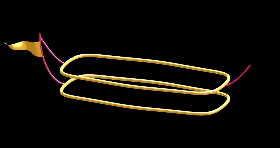
Now for some final details including the ropes to the blimp, a flag hung on one of the ropes, and railings around the walkways so that passengers don't plummet to their doom. This will make use of the ad-hoc "ropeG" function, which takes a 3D vector of points and makes a conforming cylinder around it, so that you get lighting functions etc. that don't work on simple lines. This function is added to the script at the end to do this:
% Rope function for making a 3D curve have thickness, like a rope.
% Inputs:
% - xyz (3D curve vector, M points in 3 x M format)
% - N (Number of radial points in cylinder function around the curve
% - W (Width of the rope)
%
% Outputs:
% - xf, yf, zf (Matrices that can be used with surf())
function [xf, yf, zf] = RopeG(xyz, N, W)
% Canonical cylinder with N points in circumference
[xt,yt,zt] = cylinder(1, N);
% Extract just the first ring and make (W) wide
xyzt = [xt(1, :); yt(1, :); zt(1, :)]*W;
% Get local orientation vector between adjacent points in rope
dxyz = xyz(:, 2:end) - xyz(:, 1:end-1);
dxyz(:, end+1) = dxyz(:, end);
vcs = dxyz./vecnorm(dxyz);
% We need to orient circle so that its plane normal is parallel to
% xyzt. This is a kludgey way to do that.
vcs2 = [ones(2, size(vcs, 2)); -(vcs(1, :) + vcs(2, :))./(vcs(3, :)+0.01)];
vcs2 = vcs2./vecnorm(vcs2);
vcs3 = cross(vcs, vcs2);
p = @(x)permute(x, [1, 3, 2]);
rmats = [p(vcs3), p(vcs2), p(vcs)];
% Create surface
xyzF = pagemtimes(rmats, xyzt) + permute(xyz, [1, 3, 2]);
% Outputs for surf format
xf = squeeze(xyzF(1, :, :));
yf = squeeze(xyzF(2, :, :));
zf = squeeze(xyzF(3, :, :));
end
Using this function we can define the ropes and balconies. Note that the balconies simply recycle one of the rows of the original carriage surface, defining the outer rim of the walkway, but bumping up in the z-dimension.
cb=-sqrt(1-linspace(1, 0, 100).^2)';
c1v=[linspace(-67, -51)', 0*ones(100,1),cb*30+35];
c2v=[c1v(:,1),c1v(:,2),(linspace(1,0).^1.5-1)'*15+33];
c3v=c2v.*[-1,1,1];
[xr,yr,zr]=RopeG(c1v', 10, .5);
surf(xr,yr,zr,0*xr+c2,'Parent',P);
[xr,yr,zr]=RopeG(c2v', 10, .5);
surf(xr,yr,zr,0*zr+c2,'Parent',P);
[xr,yr,zr]=RopeG(c3v', 10, .5);
surf(xr,yr,zr,0*zr+c2,'Parent',P);
% Finally, balconies would add a nice touch to the carriage keep people
% from falling to their death at 10,000 feet.
[rx,ry,rz]=RopeG([x3T(14, :); y3T(14,:); 0*x3T(14,:)+18]*1.01, 10, 1);
surf(rx,ry,rz,0*rz+cat(3,0.7,.5,.1),'Parent',P);
surf(rx,ry,rz-13,0*rz+cat(3,0.7,.5,.1),'Parent',P);
And, very last, we are going to add a flag attached to the outer cable. Let's make it flap in the wind. To make it we will recycle the z3 matrix again, but taper it based on its x-value. Then we will sinusoidally oscillate the flag in the y dimension as a function of x, constraining the y-position to be zero where it meets the cable. Lastly, we will displace it quadratically in the x-dimension as a function of z so that it lines up nicely with the rope. The phase of the sine-function is modified in the animation loop to give it a flapping motion.
h=linspace(0,1);
sc=10;
[fx,fz]=meshgrid(h,h-.5);
F=surf(sc*2.5*fx-90-2*(fz+.5).^2,sc*.3*erf(3*(1-h)).*sin(10*fx+n/5),sc*fz.*h+25,0*fx+c3,'Parent',P);
Plotting just the cables and flag shows:
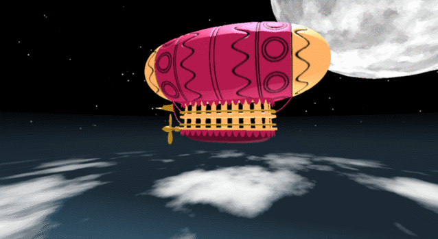
Putting all the pieces together reveals the full airship:
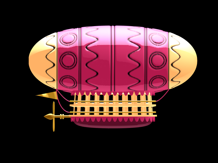
A note about lighting: lighting and material properties really change the feel of the image you create. The above picture is rendered in a cartoony style by setting the specular exponent to a very low value (1), and adding lots of diffuse and ambient reflectivity as well. A light below the airship was also added, albeit with lower strength. Settings used for this plot were:
shading flat
view([0, 0]);
L=light;
L.Color = [1,1,1]/4;
light('position', [0, 0.5, 1], 'color', [1,1,1]);
light('position', [0, 1, -1], 'color', [1, 1, 1]/5);
material([1, 1, .7, 1])
set(gcf, 'color', 'k');
axis equal off
What about all the rest of the stuff (clouds, moon, atmospheric haze etc.) These were all (mostly) recycled bits from previous minihack entries. The clouds were made using power-law noise as explained in Adam Danz' blog post. The moon was borrowed from moonrun, but with an increased number of points. Atmospheric haze was recycled from Matlon5. The rest is just camera angles, hgtransform matrix updates, and updating alpha-maps or vertex coordinates.
Finally, the use of hann() adds the signal processing toolbox as a dependency. To avoid this use the following anonymous function:
hann = @(x)-cospi(linspace(0,2,x)')/2+.5;
Hello everyone,
Over the past few weeks, our community members have shared some incredible insights and resources. Here are some highlights worth checking out:
Interesting Questions
Johnathan is seeking help with implementing a complex equation into MATLAB's curve fitting toolbox. If you have experience with curve fitting or MATLAB, your input could be invaluable!
Popular Discussions
Athanasios continues his exploration of the Duffing Equation, delving into its chaotic behavior. It's a fascinating read for anyone interested in nonlinear dynamics or chaos theory.
John shares his playful exploration with MATLAB to find a generative equation for a sequence involving Fibonacci numbers. It's an intriguing challenge for those who love mathematical puzzles.
From File Exchange
Ayesha provides a graphical analysis of linearised models in epidemiology, offering a detailed look at the dynamics of these systems. This resource is perfect for those interested in mathematical modeling.
Gareth brings some humor to MATLAB with a toolbox designed to share jokes. It's a fun way to lighten the mood during conferences or meetups.
From the Blogs
Ned Gulley interviews Tim Marston, the 2023 MATLAB Mini Hack contest winner. Tim's creativity and skills are truly inspiring, and his story is a must-read for aspiring programmers.
Sivylla discusses the integration of AI with embedded systems, highlighting the benefits of using MATLAB and Simulink. It's an insightful read for anyone interested in the future of AI technology.
Thank you to all our contributors for sharing your knowledge and creativity. We encourage everyone to engage with these posts and continue fostering a vibrant and supportive community.
Happy exploring!
Explore the newest online training courses, available as of 2024b: one new Onramp, eight new short courses, and one new learning path. Yes, that’s 10 new offerings. We’ve been busy.
As a reminder, Onramps are free to all. Short courses and learning paths require a subscription to the Online Training Suite (OTS).
- Multibody Simulation Onramp
- Analyzing Results in Simulink
- Battery Pack Modeling
- Introduction to Motor Control
- Signal Processing Techniques for Streaming Signals
- Core Signal Processing Techniques in MATLAB (learning path – includes the four short courses listed below)
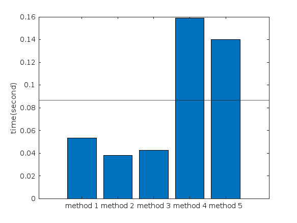
Create a struct arrays where each struct has field names "a," "b," and "c," which store different types of data. What efficient methods do you have to assign values from individual variables "a," "b," and "c" to each struct element? Here are five methods I've provided, listed in order of decreasing efficiency. What do you think?
Create an array of 10,000 structures, each containing each of the elements corresponding to the a,b,c variables.
num = 10000;
a = (1:num)';
b = string(a);
c = rand(3,3,num);
Here are the methods;
%% method1
t1 =tic;
s = struct("a",[], ...
"b",[], ...
"c",[]);
s1 = repmat(s,num,1);
for i = 1:num
s1(i).a = a(i);
s1(i).b = b(i);
s1(i).c = c(:,:,i);
end
t1 = toc(t1);
%% method2
t2 =tic;
for i = num:-1:1
s2(i).a = a(i);
s2(i).b = b(i);
s2(i).c = c(:,:,i);
end
t2 = toc(t2);
%% method3
t3 =tic;
for i = 1:num
s3(i).a = a(i);
s3(i).b = b(i);
s3(i).c = c(:,:,i);
end
t3 = toc(t3);
%% method4
t4 =tic;
ct = permute(c,[3,2,1]);
t = table(a,b,ct);
s4 = table2struct(t);
t4 = toc(t4);
%% method5
t5 =tic;
s5 = struct("a",num2cell(a),...
"b",num2cell(b),...
"c",squeeze(mat2cell(c,3,3,ones(num,1))));
t5 = toc(t5);
%% plot
bar([t1,t2,t3,t4,t5])
xtickformat('method %g')
ylabel("time(second)")
yline(mean([t1,t2,t3,t4,t5]))
您也可以从以下列表中选择网站:
美洲
- América Latina (Español)
- Canada (English)
- United States (English)
欧洲
- Belgium (English)
- Denmark (English)
- Deutschland (Deutsch)
- España (Español)
- Finland (English)
- France (Français)
- Ireland (English)
- Italia (Italiano)
- Luxembourg (English)
- Netherlands (English)
- Norway (English)
- Österreich (Deutsch)
- Portugal (English)
- Sweden (English)
- Switzerland
- United Kingdom(English)
亚太
- Australia (English)
- India (English)
- New Zealand (English)
- 中国
- 日本Japanese (日本語)
- 한국Korean (한국어)