主要内容
Results for
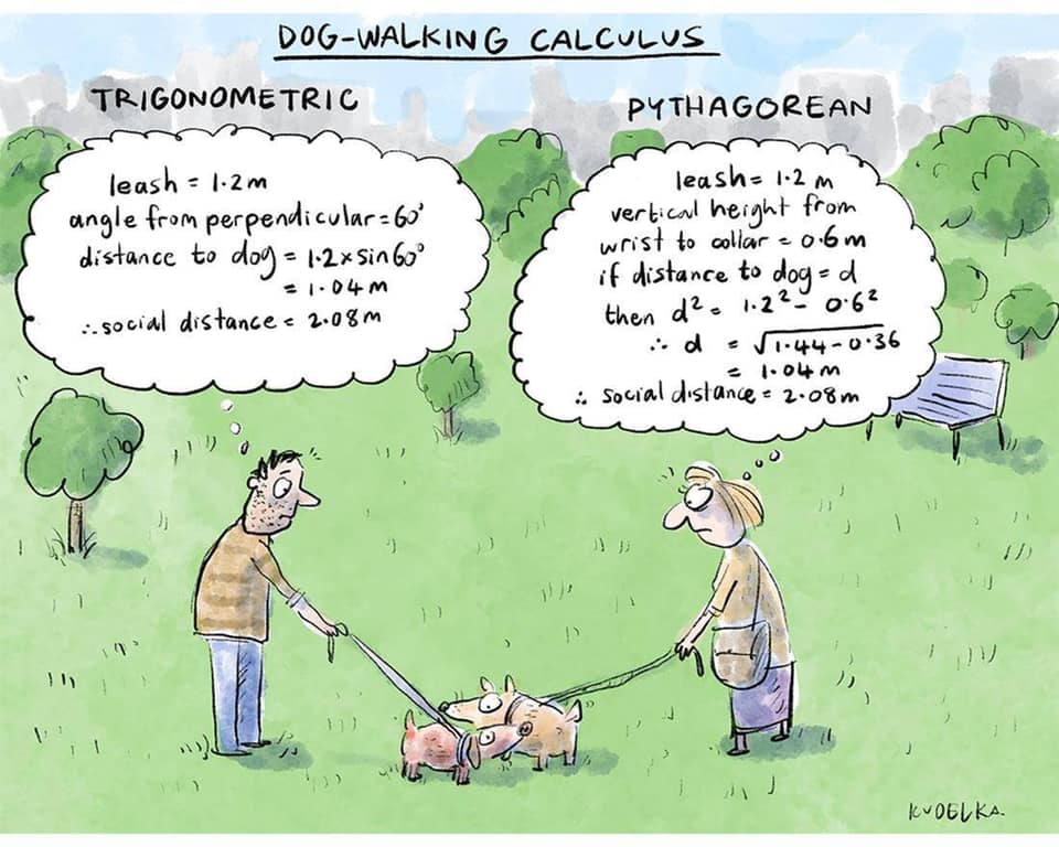
What's your way?
I created an ellipse visualizer in #MATLAB using App Designer! To read more about it, and how it ties to the recent total solar eclipse, check out my latest blog post:
Github Repo of the app (you can open it on MATLAB Online!):
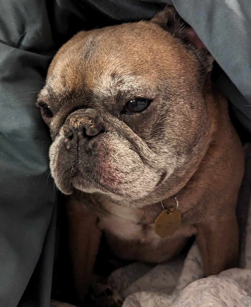
Mari is helping Dad work.
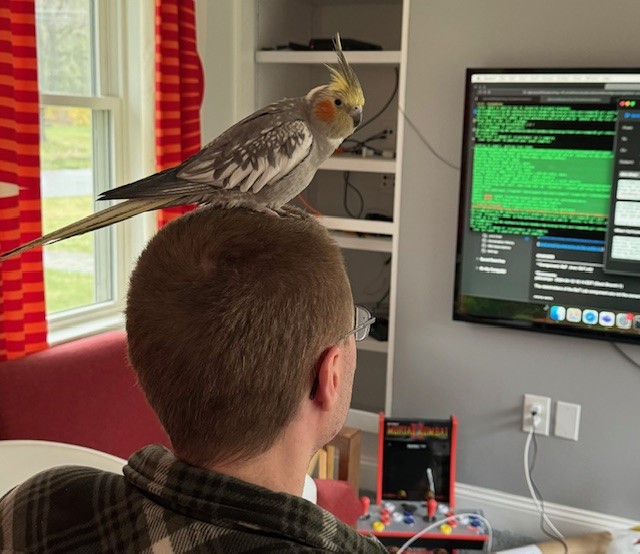
Today, he got dressed for work to design some new dog toy-making algorithms. #nationalpetday

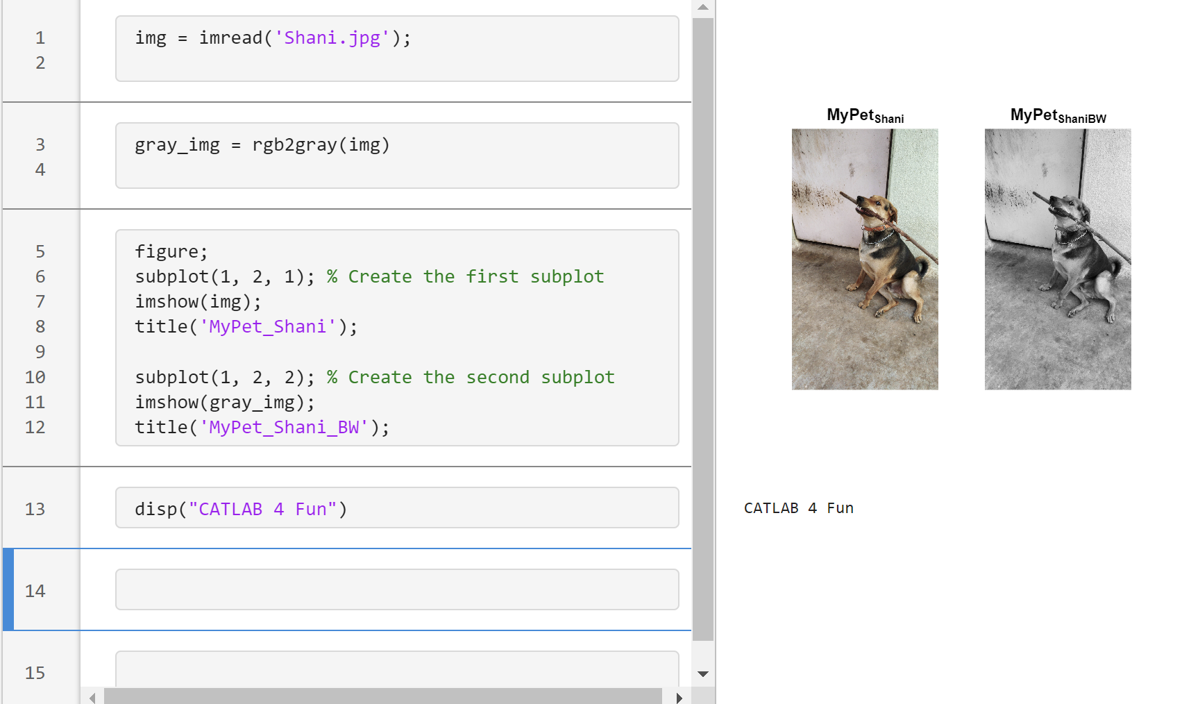
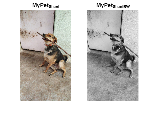
Transforming my furry friend into a grayscale masterpiece with MATLAB! 🐾 #MATLABPetsDay ✌️
This is Stella while waiting to see if the code works...
What's the weather like in your place?
I'm excited to share some valuable resources that I've found to be incredibly helpful for anyone looking to enhance their MATLAB skills. Whether you're just starting out, studying as a student, or are a seasoned professional, these guides and books offer a wealth of information to aid in your learning journey.
These materials are freely available and can be a great addition to your learning resources. They cover a wide range of topics and are designed to help users at all levels to improve their proficiency in MATLAB.
Happy learning and I hope you find these resources as useful as I have!
I found this link posted on Reddit.
https://workhunty.com/job-blog/where-is-the-best-place-to-be-a-programmer/Matlab/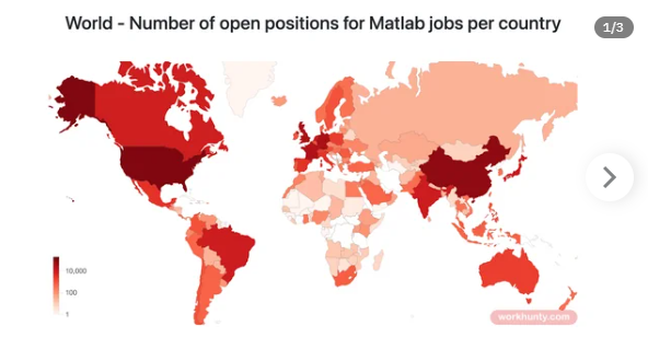
Let S be the closed surface composed of the hemisphere 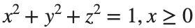 and the base
 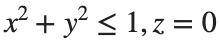 Let
Let  be the electric field defined by
 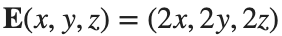 . Find the electric flux through S. (Hint: Divide S into two parts and calculate
 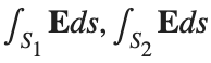 ).
).
% Define the limits of integration for the hemisphere S1
theta_lim = [-pi/2, pi/2];
phi_lim = [0, pi/2];
% Perform the double integration over the spherical surface of the hemisphere S1
% Define the electric flux function for the hemisphere S1
flux_function_S1 = @(theta, phi) 2 * sin(phi);
electric_flux_S1 = integral2(flux_function_S1, theta_lim(1), theta_lim(2), phi_lim(1), phi_lim(2));
% For the base of the hemisphere S2, the electric flux is 0 since the electric
% field has no z-component at the base
electric_flux_S2 = 0;
% Calculate the total electric flux through the closed surface S
total_electric_flux = electric_flux_S1 + electric_flux_S2;
% Display the flux calculations
disp(['Electric flux through the hemisphere S1: ', num2str(electric_flux_S1)]);
disp(['Electric flux through the base of the hemisphere S2: ', num2str(electric_flux_S2)]);
disp(['Total electric flux through the closed surface S: ', num2str(total_electric_flux)]);
% Parameters for the plot
radius = 1; % Radius of the hemisphere
% Create a meshgrid for theta and phi for the plot
[theta, phi] = meshgrid(linspace(theta_lim(1), theta_lim(2), 20), linspace(phi_lim(1), phi_lim(2), 20));
% Calculate Cartesian coordinates for the points on the hemisphere
x = radius * sin(phi) .* cos(theta);
y = radius * sin(phi) .* sin(theta);
z = radius * cos(phi);
% Define the electric field components
Ex = 2 * x;
Ey = 2 * y;
Ez = 2 * z;
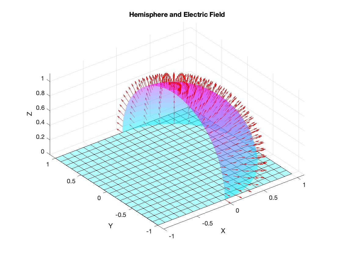
% Plot the hemisphere
figure;
surf(x, y, z, 'FaceAlpha', 0.5, 'EdgeColor', 'none');
hold on;
% Plot the electric field vectors
quiver3(x, y, z, Ex, Ey, Ez, 'r');
% Plot the base of the hemisphere
[x_base, y_base] = meshgrid(linspace(-radius, radius, 20), linspace(-radius, radius, 20));
z_base = zeros(size(x_base));
surf(x_base, y_base, z_base, 'FaceColor', 'cyan', 'FaceAlpha', 0.3);
% Additional plot settings
colormap('cool');
axis equal;
grid on;
xlabel('X');
ylabel('Y');
zlabel('Z');
title('Hemisphere and Electric Field');
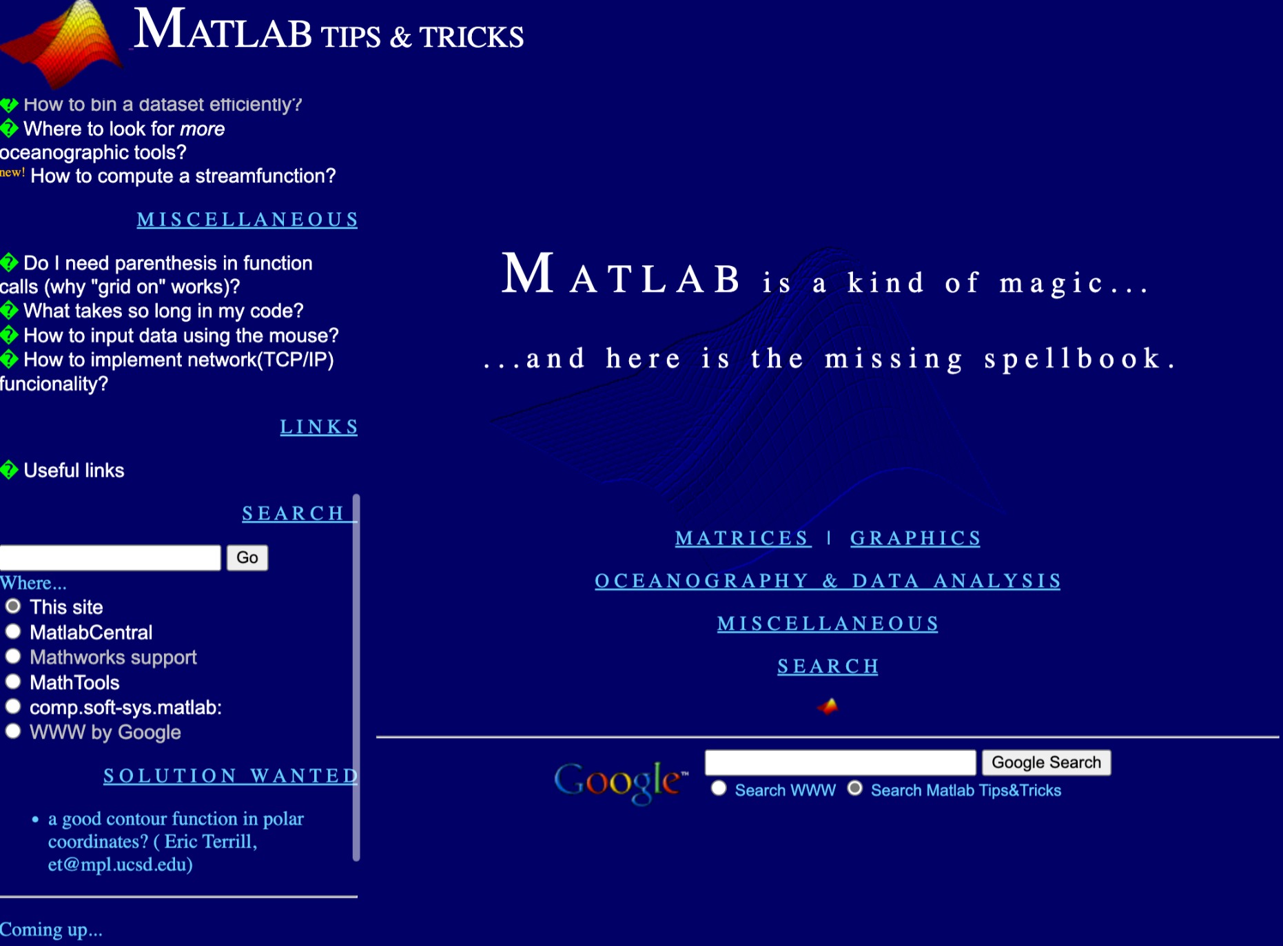
I feel like no one at UC San Diego knows this page, let alone this server, is still live. For the younger generation, this is what the whole internet used to look like :)
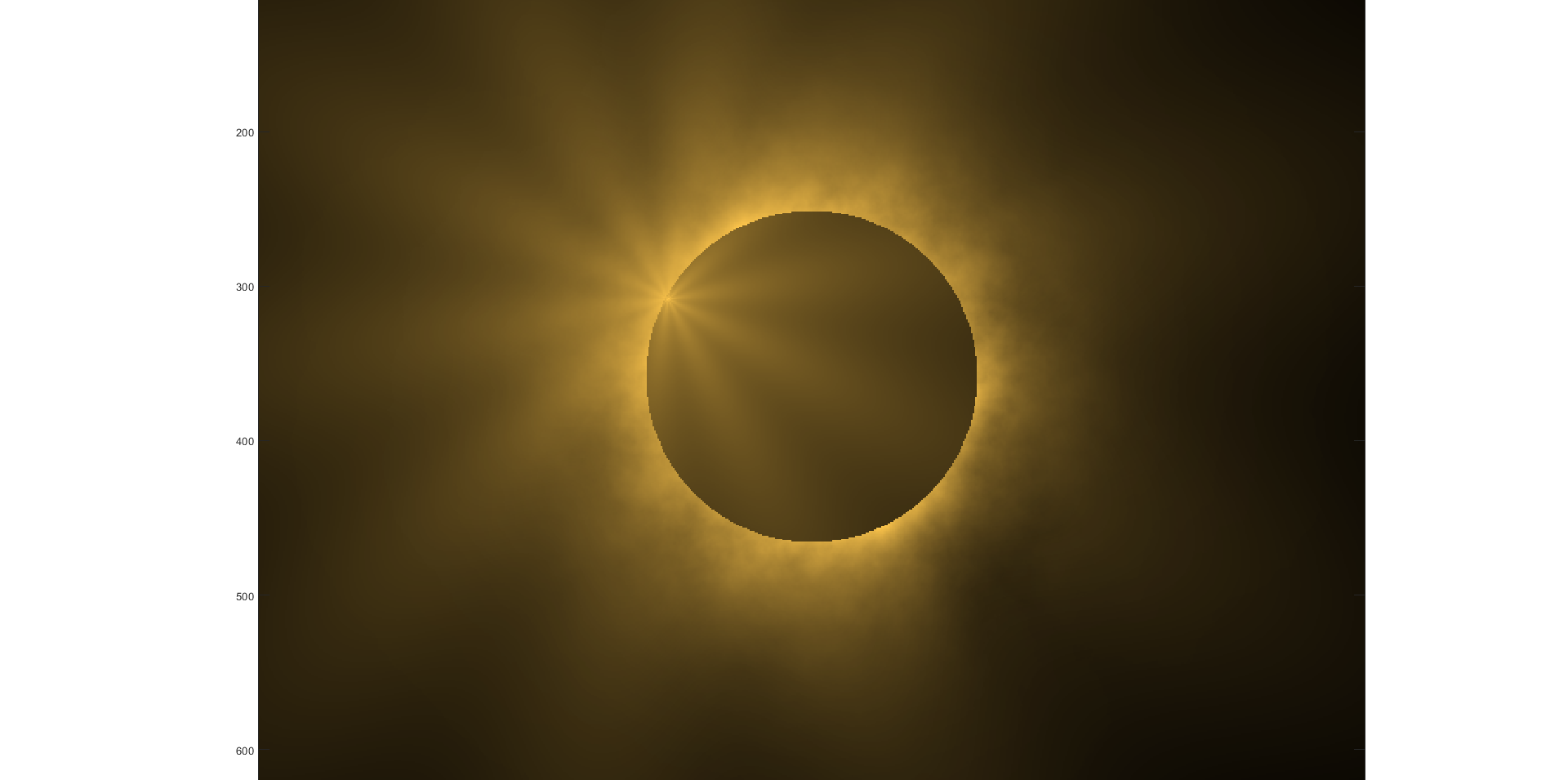
Although, I think I will only get to see a partial eclipse (April 8th!) from where I am at in the U.S. I will always have MATLAB to make my own solar eclipse. Just as good as the real thing.
Code (found on the @MATLAB instagram)
a=716;
v=255;
X=linspace(-10,10,a);
[~,r]=cart2pol(X,X');
colormap(gray.*[1 .78 .3]);
[t,g]=cart2pol(X+2.6,X'+1.4);
image(rescale(-1*(2*sin(t*10)+60*g.^.2),0,v))
hold on
h=exp(-(r-3)).*abs(ifft2(r.^-1.8.*cos(7*rand(a))));
h(r<3)=0;
image(v*ones(a),'AlphaData',rescale(h,0,1))
camva(3.8)
One of the privileges of working at MathWorks is that I get to hang out with some really amazing people. Steve Eddins, of ‘Steve on Image Processing’ fame is one of those people. He recently announced his retirement and before his final day, I got the chance to interview him. See what he had to say over at The MATLAB Blog The Steve Eddins Interview: 30 years of MathWorking
Before we begin, you will need to make sure you have 'sir_age_model.m' installed. Once you've downloaded this folder into your working directory, which can be located at your current folder. If you can see this file in your current folder, then it's safe to use it. If you choose to use MATLAB online or MATLAB Mobile, you may upload this to your MATLAB Drive.
This is the code for the SIR model stratified into 2 age groups (children and adults). For a detailed explanation of how to derive the force of infection by age group.
% Main script to run the SIR model simulation
% Initial state values
initial_state_values = [200000; 1; 0; 800000; 0; 0]; % [S1; I1; R1; S2; I2; R2]
% Parameters
parameters = [0.05; 7; 6; 1; 10; 1/5]; % [b; c_11; c_12; c_21; c_22; gamma]
% Time span for the simulation (3 months, with daily steps)
tspan = [0 90];
% Solve the ODE
[t, y] = ode45(@(t, y) sir_age_model(t, y, parameters), tspan, initial_state_values);
% Plotting the results
plot(t, y);
xlabel('Time (days)');
ylabel('Number of people');
legend('S1', 'I1', 'R1', 'S2', 'I2', 'R2');
title('SIR Model with Age Structure');
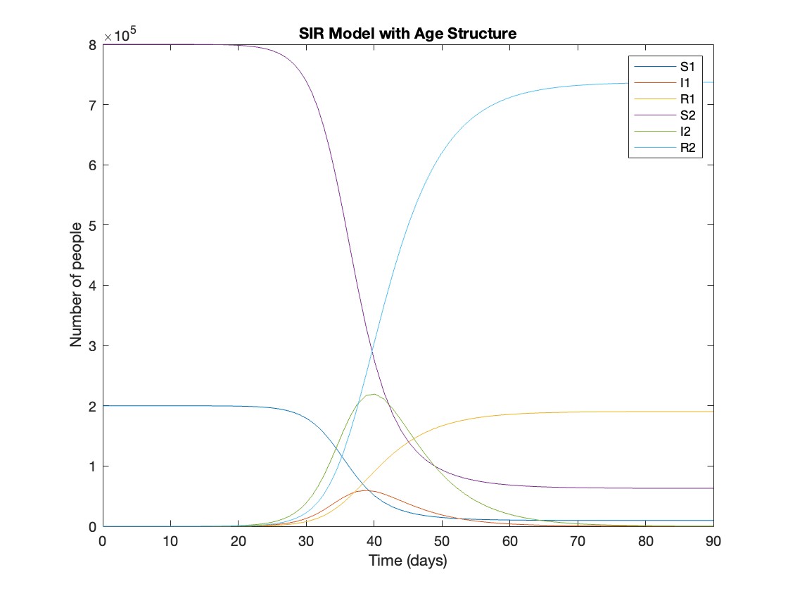
What was the cumulative incidence of infection during this epidemic? What proportion of those infections occurred in children?
In the SIR model, the cumulative incidence of infection is simply the decline in susceptibility.
% Assuming 'y' contains the simulation results from the ode45 function
% and 't' contains the time points
% Total cumulative incidence
total_cumulative_incidence = (y(1,1) - y(end,1)) + (y(1,4) - y(end,4));
fprintf('Total cumulative incidence: %f\n', total_cumulative_incidence);
% Cumulative incidence in children
cumulative_incidence_children = (y(1,1) - y(end,1));
% Proportion of infections in children
proportion_infections_children = cumulative_incidence_children / total_cumulative_incidence;
fprintf('Proportion of infections in children: %f\n', proportion_infections_children);
927,447 people became infected during this epidemic, 20.5% of which were children.
Which age group was most affected by the epidemic?
To answer this, we can calculate the proportion of children and adults that became infected.
% Assuming 'y' contains the simulation results from the ode45 function
% and 't' contains the time points
% Proportion of children that became infected
initial_children = 200000; % initial number of susceptible children
final_susceptible_children = y(end,1); % final number of susceptible children
proportion_infected_children = (initial_children - final_susceptible_children) / initial_children;
fprintf('Proportion of children that became infected: %f\n', proportion_infected_children);
% Proportion of adults that became infected
initial_adults = 800000; % initial number of susceptible adults
final_susceptible_adults = y(end,4); % final number of susceptible adults
proportion_infected_adults = (initial_adults - final_susceptible_adults) / initial_adults;
fprintf('Proportion of adults that became infected: %f\n', proportion_infected_adults);
Throughout this epidemic, 95% of all children and 92% of all adults were infected. Children were therefore slightly more affected in proportion to their population size, even though the majority of infections occurred in adults.
Are you going to be in the path of totality? How can you predict, track, and simulate the solar eclipse using MATLAB?
In one line of MATLAB code, compute how far you can see at the seashore. In otherwords, how far away is the horizon from your eyes? You can assume you know your height and the diameter or radius of the earth.
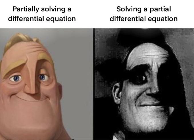
Keep calm and study PDEs
Me at the beginning of every meeting

A bit late. Compliments to Chris for sharing.
The latest release is pretty much upon us. Official annoucements will be coming soon and the eagle-eyed among you will have started to notice some things shifting around on the MathWorks website as we ready for this.
The pre-release has been available for a while. Maybe you've played with it? I have...I've even been quietly using it to write some of my latest blog posts...and I have several queued up for publication after MathWorks officially drops the release.
At the time of writing, this page points to the pre-release highlights. Prerelease Release Highlights - MATLAB & Simulink (mathworks.com)
What excites you about this release? why?
您也可以从以下列表中选择网站:
美洲
- América Latina (Español)
- Canada (English)
- United States (English)
欧洲
- Belgium (English)
- Denmark (English)
- Deutschland (Deutsch)
- España (Español)
- Finland (English)
- France (Français)
- Ireland (English)
- Italia (Italiano)
- Luxembourg (English)
- Netherlands (English)
- Norway (English)
- Österreich (Deutsch)
- Portugal (English)
- Sweden (English)
- Switzerland
- United Kingdom(English)
亚太
- Australia (English)
- India (English)
- New Zealand (English)
- 中国
- 日本Japanese (日本語)
- 한국Korean (한국어)