主要内容

Results for


goc3
goc3
Last activity 2024-9-8,14:47

Base case:
Suppose you need to do a computation many times. We are going to assume that this computation cannot be vectorized. The simplest case is to use a for loop:
number_of_elements = 1e6;
test_fcn = @(x) sqrt(x) / x;
tic
for i = 1:number_of_elements
x(i) = test_fcn(i);
end
t_forward = toc;
disp(t_forward + " seconds")
0.10925 seconds
Preallocation:
This can easily be sped up by preallocating the variable that houses results:
tic
x = zeros(number_of_elements, 1);
for i = 1:number_of_elements
x(i) = test_fcn(i);
end
t_forward_prealloc = toc;
disp(t_forward_prealloc + " seconds")
0.035106 seconds
In this example, preallocation speeds up the loop by a factor of about three to four (running in R2024a). Comment below if you get dramatically different results.
disp(sprintf("%.1f", t_forward / t_forward_prealloc))
3.1
Run it in reverse:
Is there a way to skip the explicit preallocation and still be fast? Indeed, there is.
clear x
tic
for i = number_of_elements:-1:1
x(i) = test_fcn(i);
end
t_backward = toc;
disp(t_backward + " seconds")
0.032392 seconds
By running the loop backwards, the preallocation is implicitly performed during the first iteration and the loop runs in about the same time (within statistical noise):
disp(sprintf("%.2f", t_forward_prealloc / t_backward))
1.08
Do you get similar results when running this code? Let us know your thoughts in the comments below.
Beneficial side effect:
Have you ever had to use a for loop to delete elements from a vector? If so, keeping track of index offsets can be tricky, as deleting any element shifts all those that come after. By running the for loop in reverse, you don't need to worry about index offsets while deleting elements.
The Ans Hack is a dubious way to shave a few points off your solution score. Instead of a standard answer like this
function y = times_two(x)
y = 2*x;
end
you would do this
function ans = times_two(x)
2*x;
end
The ans variable is automatically created when there is no left-hand side to an evaluated expression. But it makes for an ugly function. I don't think anyone actually defends it as a good practice. The question I would ask is: is it so offensive that it should be specifically disallowed by the rules? Or is it just one of many little hacks that you see in Cody, inelegant but tolerable in the context of the surrounding game?
Incidentally, I wrote about the Ans Hack long ago on the Community Blog. Dealing with user-unfriendly code is also one of the reasons we created the Head-to-Head voting feature. Some techniques are good for your score, and some are good for your code readability. You get to decide with you care about.
Many times when ploting, we not only need to set the color of the plot, but also its
transparency, Then how we set the alphaData of colorbar at the same time ?
It seems easy to do so :
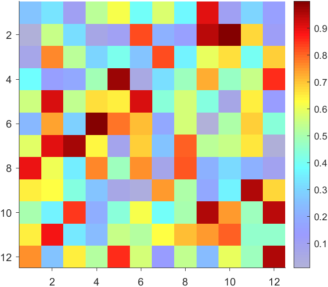
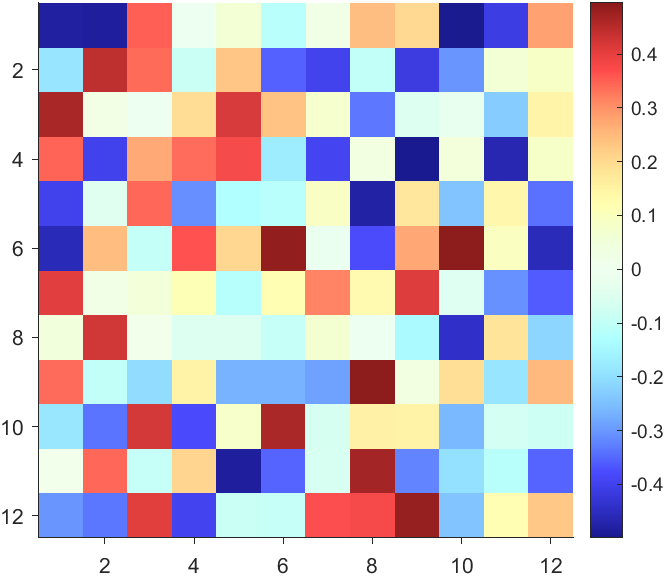
data = rand(12,12);
% Transparency range 0-1, .3-1 for better appearance here
AData = rescale(- data, .3, 1);
% Draw an imagesc with numerical control over colormap and transparency
imagesc(data, 'AlphaData',AData);
colormap(jet);
ax = gca;
ax.DataAspectRatio = [1,1,1];
ax.TickDir = 'out';
ax.Box = 'off';
% get colorbar object
CBarHdl = colorbar;
pause(1e-16)
% Modify the transparency of the colorbar
CData = CBarHdl.Face.Texture.CData;
ALim = [min(min(AData)), max(max(AData))];
CData(4,:) = uint8(255.*rescale(1:size(CData, 2), ALim(1), ALim(2)));
CBarHdl.Face.Texture.ColorType = 'TrueColorAlpha';
CBarHdl.Face.Texture.CData = CData;
But !!!!!!!!!!!!!!! We cannot preserve the changes when saving them as images :
It seems that when saving plots, the `Texture` will be refresh, but the `Face` will not :
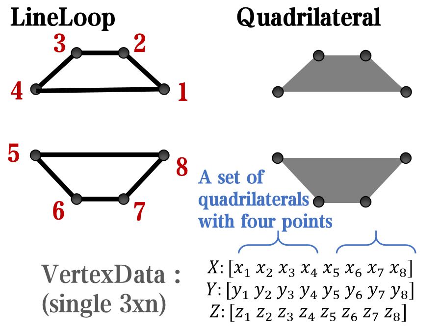
however, object Face only have 4 colors to change(The four corners of a quadrilateral), how
can we set more colors ??
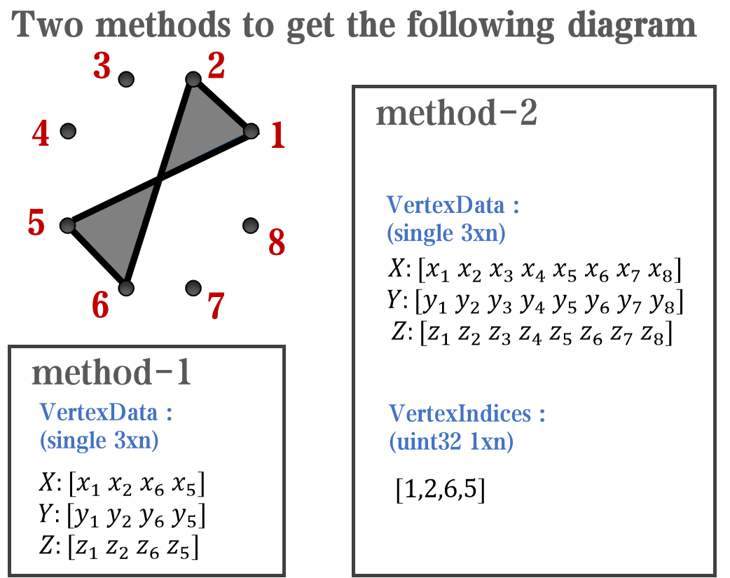
`Face` is a quadrilateral object, and we can change the `VertexData` to draw more than one little quadrilaterals:
data = rand(12,12);
% Transparency range 0-1, .3-1 for better appearance here
AData = rescale(- data, .3, 1);
%Draw an imagesc with numerical control over colormap and transparency
imagesc(data, 'AlphaData',AData);
colormap(jet);
ax = gca;
ax.DataAspectRatio = [1,1,1];
ax.TickDir = 'out';
ax.Box = 'off';
% get colorbar object
CBarHdl = colorbar;
pause(1e-16)
% Modify the transparency of the colorbar
CData = CBarHdl.Face.Texture.CData;
ALim = [min(min(AData)), max(max(AData))];
CData(4,:) = uint8(255.*rescale(1:size(CData, 2), ALim(1), ALim(2)));
warning off
CBarHdl.Face.ColorType = 'TrueColorAlpha';
VertexData = CBarHdl.Face.VertexData;
tY = repmat((1:size(CData,2))./size(CData,2), [4,1]);
tY1 = tY(:).'; tY2 = tY - tY(1,1); tY2(3:4,:) = 0; tY2 = tY2(:).';
tM1 = [tY1.*0 + 1; tY1; tY1.*0 + 1];
tM2 = [tY1.*0; tY2; tY1.*0];
CBarHdl.Face.VertexData = repmat(VertexData, [1,size(CData,2)]).*tM1 + tM2;
CBarHdl.Face.ColorData = reshape(repmat(CData, [4,1]), 4, []);
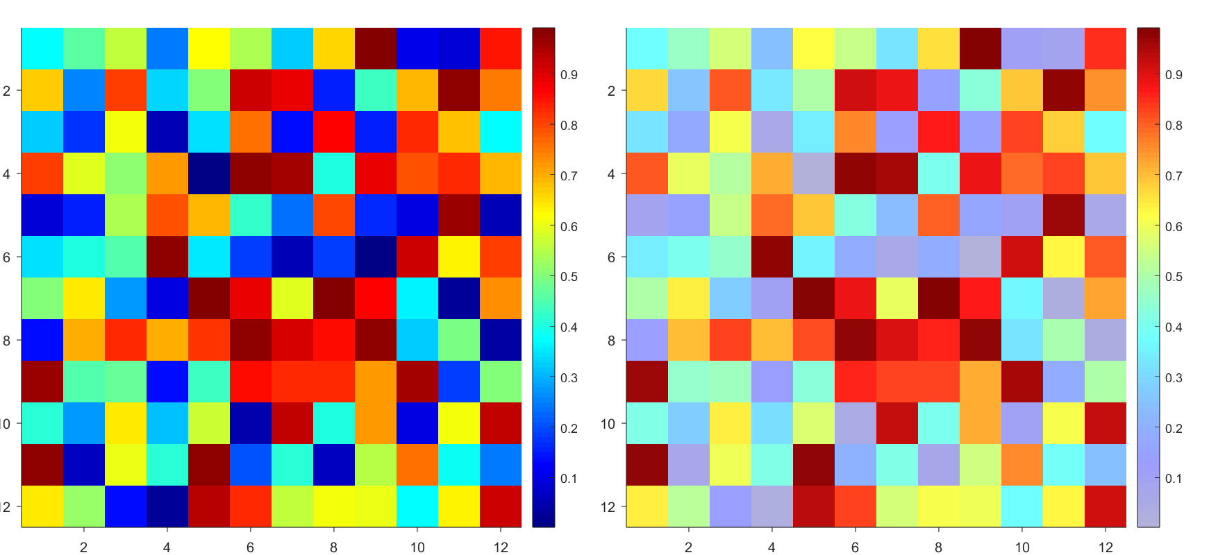
The higher the value, the more transparent it becomes
data = rand(12,12);
AData = rescale(- data, .3, 1);
imagesc(data, 'AlphaData',AData);
colormap(jet);
ax = gca;
ax.DataAspectRatio = [1,1,1];
ax.TickDir = 'out';
ax.Box = 'off';
CBarHdl = colorbar;
pause(1e-16)
CData = CBarHdl.Face.Texture.CData;
ALim = [min(min(AData)), max(max(AData))];
CData(4,:) = uint8(255.*rescale(size(CData, 2):-1:1, ALim(1), ALim(2)));
warning off
CBarHdl.Face.ColorType = 'TrueColorAlpha';
VertexData = CBarHdl.Face.VertexData;
tY = repmat((1:size(CData,2))./size(CData,2), [4,1]);
tY1 = tY(:).'; tY2 = tY - tY(1,1); tY2(3:4,:) = 0; tY2 = tY2(:).';
tM1 = [tY1.*0 + 1; tY1; tY1.*0 + 1];
tM2 = [tY1.*0; tY2; tY1.*0];
CBarHdl.Face.VertexData = repmat(VertexData, [1,size(CData,2)]).*tM1 + tM2;
CBarHdl.Face.ColorData = reshape(repmat(CData, [4,1]), 4, []);
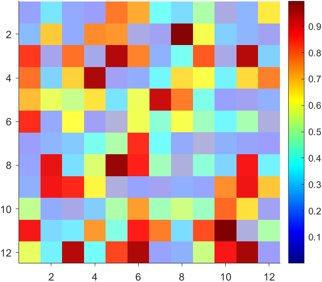
More transparent in the middle
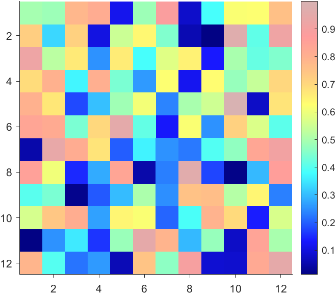
data = rand(12,12) - .5;
AData = rescale(abs(data), .1, .9);
imagesc(data, 'AlphaData',AData);
colormap(jet);
ax = gca;
ax.DataAspectRatio = [1,1,1];
ax.TickDir = 'out';
ax.Box = 'off';
CBarHdl = colorbar;
pause(1e-16)
CData = CBarHdl.Face.Texture.CData;
ALim = [min(min(AData)), max(max(AData))];
CData(4,:) = uint8(255.*rescale(abs((1:size(CData, 2)) - (1 + size(CData, 2))/2), ALim(1), ALim(2)));
warning off
CBarHdl.Face.ColorType = 'TrueColorAlpha';
VertexData = CBarHdl.Face.VertexData;
tY = repmat((1:size(CData,2))./size(CData,2), [4,1]);
tY1 = tY(:).'; tY2 = tY - tY(1,1); tY2(3:4,:) = 0; tY2 = tY2(:).';
tM1 = [tY1.*0 + 1; tY1; tY1.*0 + 1];
tM2 = [tY1.*0; tY2; tY1.*0];
CBarHdl.Face.VertexData = repmat(VertexData, [1,size(CData,2)]).*tM1 + tM2;
CBarHdl.Face.ColorData = reshape(repmat(CData, [4,1]), 4, []);
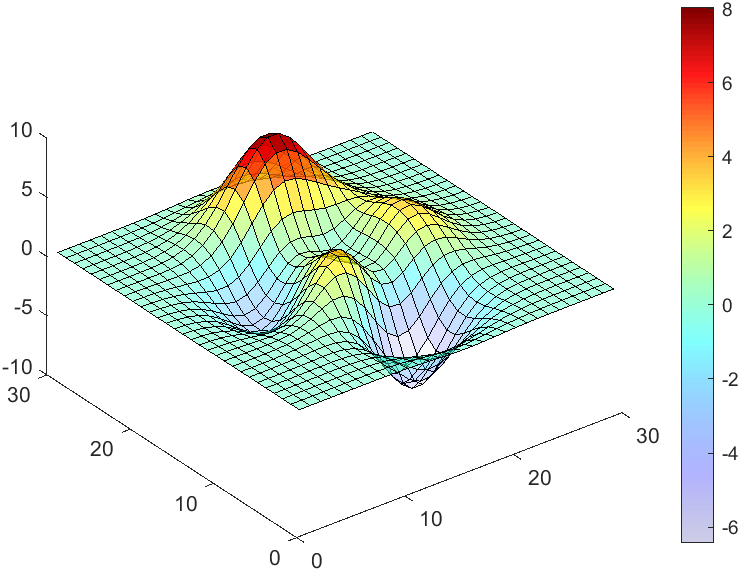
The code will work if the plot have AlphaData property
data = peaks(30);
AData = rescale(data, .2, 1);
surface(data, 'FaceAlpha','flat','AlphaData',AData);
colormap(jet(100));
ax = gca;
ax.DataAspectRatio = [1,1,1];
ax.TickDir = 'out';
ax.Box = 'off';
view(3)
CBarHdl = colorbar;
pause(1e-16)
CData = CBarHdl.Face.Texture.CData;
ALim = [min(min(AData)), max(max(AData))];
CData(4,:) = uint8(255.*rescale(1:size(CData, 2), ALim(1), ALim(2)));
warning off
CBarHdl.Face.ColorType = 'TrueColorAlpha';
VertexData = CBarHdl.Face.VertexData;
tY = repmat((1:size(CData,2))./size(CData,2), [4,1]);
tY1 = tY(:).'; tY2 = tY - tY(1,1); tY2(3:4,:) = 0; tY2 = tY2(:).';
tM1 = [tY1.*0 + 1; tY1; tY1.*0 + 1];
tM2 = [tY1.*0; tY2; tY1.*0];
CBarHdl.Face.VertexData = repmat(VertexData, [1,size(CData,2)]).*tM1 + tM2;
CBarHdl.Face.ColorData = reshape(repmat(CData, [4,1]), 4, []);
There are a host of problems on Cody that require manipulation of the digits of a number. Examples include summing the digits of a number, separating the number into its powers, and adding very large numbers together.
If you haven't come across this trick yet, you might want to write it down (or save it electronically):
digits = num2str(4207) - '0'
That code results in the following:
digits =
4 2 0 7
Now, summing the digits of the number is easy:
sum(digits)
ans =
13
Hello and a warm welcome to everyone! We're excited to have you in the Cody Discussion Channel. To ensure the best possible experience for everyone, it's important to understand the types of content that are most suitable for this channel.
Content that belongs in the Cody Discussion Channel:
  • Tips & tricks: Discuss strategies for solving Cody problems that you've found effective.
  • Ideas or suggestions for improvement: Have thoughts on how to make Cody better? We'd love to hear them.
  • Issues: Encountering difficulties or bugs with Cody? Let us know so we can address them.
  • Requests for guidance: Stuck on a Cody problem? Ask for advice or hints, but make sure to show your efforts in attempting to solve the problem first.
  • General discussions: Anything else related to Cody that doesn't fit into the above categories.
Content that does not belong in the Cody Discussion Channel:
  • Comments on specific Cody problems: Examples include unclear problem descriptions or incorrect testing suites.
  • Comments on specific Cody solutions: For example, you find a solution creative or helpful.
Please direct such comments to the Comments section on the problem or solution page itself.
We hope the Cody discussion channel becomes a vibrant space for sharing expertise, learning new skills, and connecting with others.
How to leave feedback on a doc page
Leaving feedback is a two-step process. At the bottom of most pages in the MATLAB documentation is a star rating.
Start by selecting a star that best answers the question. After selecting a star rating, an edit box appears where you can offer specific feedback.
When you press "Submit" you'll see the confirmation dialog below. You cannot go back and edit your content, although you can refresh the page to go through that process again.
Tips on leaving feedback
  • Be productive. The reader should clearly understand what action you'd like to see, what was unclear, what you think needs work, or what areas were really helpful.
  • Positive feedback is also helpful. By nature, feedback often focuses on suggestions for changes but it also helps to know what was clear and what worked well.
  • Point to specific areas of the page. This helps the reader to narrow the focus of the page to the area described by your feedback.
What happens to that feedback?
Before working at MathWorks I often left feedback on documentation pages but I never knew what happens after that. One day in 2021 I shared my speculation on the process:
> That feedback is received by MathWorks Gnomes which are never seen nor heard but visit the MathWorks documentation team at night while they are sleeping and whisper selected suggestions into their ears to manipulate their dreams. Occassionally this causes them to wake up with a Eureka moment that leads to changes in the documentation.
I'd like to let you in on the secret which is much less fanciful. Feedback left in the star rating and edit box are collected and periodically reviewed by the doc writers who look for trends on highly trafficked pages and finer grain feedback on less visited pages. Your feedback is important and often results in improvements.
David
David
Last activity 2024-5-23

A colleague said that you can search the Help Center using the phrase 'Introduced in' followed by a release version. Such as, 'Introduced in R2022a'. Doing this yeilds search results specific for that release.
Seems pretty handy so I thought I'd share.
Bringing the beauty of MathWorks Natick's tulips to life through code!
Remix challenge: create and share with us your new breeds of MATLAB tulips!
Chen Lin
Chen Lin
Last activity 2024-7-3

Northern lights captured from this weekend at MathWorks campus ✨
Did you get a chance to see lights and take some photos?
From Alpha Vantage's website: API Documentation | Alpha Vantage
Try using the built-in Matlab function webread(URL)... for example:
% copy a URL from the examples on the site
URL = 'https://www.alphavantage.co/query?function=TIME_SERIES_DAILY&symbol=IBM&apikey=demo'
% or use the pattern to create one
tickers = [{'IBM'} {'SPY'} {'DJI'} {'QQQ'}]; i = 1;
URL = ...
['https://www.alphavantage.co/query?function=TIME_SERIES_DAILY_ADJUSTED&outputsize=full&symbol=', ...
+ tickers{i}, ...
+ '&apikey=***Put Your API Key here***'];
X = webread(URL);
You can access any of the data available on the site as per the Alpha Vantage documentation using these two lines of code but with different designations for the requested data as per the documentation.
It's fun!
Dear MATLAB contest enthusiasts,
I believe many of you have been captivated by the innovative entries from Zhaoxu Liu / slanderer, in the 2023 MATLAB Flipbook Mini Hack contest.
Ever wondered about the person behind these creative entries? What drives a MATLAB user to such levels of skill? And what inspired his participation in the contest? We were just as curious as you are!
We were delighted to catch up with him and learn more about his use of MATLAB. The interview has recently been published in MathWorks Blogs. For an in-depth look into his insights and experiences, be sure to read our latest blog post: Community Q&A – Zhaoxu Liu.
But the conversation doesn't end here! Who would you like to see featured in our next interview? Drop their name in the comments section below and let us know who we should reach out to next!
Temporary print statements are often helpful during debugging but it's easy to forget to remove the statements or sometimes you may not have writing privileges for the file. This tip uses conditional breakpoints to add print statements without ever editing the file!
What are conditional breakpoints?
Conditional breakpoints allow you to write a conditional statement that is executed when the selected line is hit and if the condition returns true, MATLAB pauses at that line. Otherwise, it continues.
The Hack: use ~fprintf() as the condition
fprintf prints information to the command window and returns the size of the message in bytes. The message size will always be greater than 0 which will always evaluate as true when converted to logical. Therefore, by negating an fprintf statement within a conditional breakpoint, the fprintf command will execute, print to the command window, and evalute as false which means the execution will continue uninterupted!
How to set a conditional break point
1. Right click the line number where you want the condition to be evaluated and select "Set Conditional Breakpoint"
2. Enter a valid MATLAB expression that returns a logical scalar value in the editor dialog.
Handy one-liners
Check if a line is reached: Don't forget the negation (~) and the line break (\n)!
~fprintf('Entered callback function\n')
Display the call stack from the break point line: one of my favorites!
~fprintf('%s\n',formattedDisplayText(struct2table(dbstack)))
Inspect variable values: For scalar values,
~fprintf('v = %.5f\n', v)
Use formattedDisplayText to convert more complex data to a string
~fprintf('%s\n', formattedDisplayText(v)).
Make sense of frequent hits: In some situations such as responses to listeners or interactive callbacks, a line can be executed 100s of times per second. Incorporate a timestamp to differentiate messages during rapid execution.
~fprintf('WindowButtonDownFcn - %s\n', datetime('now'))
Closing
This tip not only keeps your code clean but also offers a dynamic way to monitor code execution and variable states without permanent modifications. Interested in digging deeper? @Steve Eddins takes this tip to the next level with his Code Trace for MATLAB tool available on the File Exchange (read more).
Summary animation
To reproduce the events in this animation:
% buttonDownFcnDemo.m
fig = figure();
tcl = tiledlayout(4,4,'TileSpacing','compact');
for i = 1:16
ax = nexttile(tcl);
title(ax,"#"+string(i))
ax.ButtonDownFcn = @axesButtonDownFcn;
xlim(ax,[-1 1])
ylim(ax,[-1,1])
hold(ax,'on')
end
function axesButtonDownFcn(obj,event)
colors = lines(16);
plot(obj,event.IntersectionPoint(1),event.IntersectionPoint(2),...
'ko','MarkerFaceColor',colors(obj.Layout.Tile,:))
end

Hello MathWorks Community,

I am excited to announce that I am currently working on a book project centered around Matrix Algebra, specifically designed for MATLAB users. This book aims to cater to undergraduate students in engineering, where Matrix Algebra serves as a foundational element.

Matrix Algebra is not only pivotal in understanding complex engineering concepts but also in applying these principles effectively in various technological solutions. MATLAB, renowned for its powerful computational capabilities, is an excellent tool to explore and implement these concepts, making it a perfect companion for this book.

As I embark on this journey to create a resource that bridges theoretical matrix algebra with practical MATLAB applications, I am looking for one or two knowledgeable individuals who have a firm grasp of both subjects. If you have experience in teaching or applying matrix algebra in engineering contexts and are familiar with MATLAB, your contribution could be invaluable.

Collaborators will help in shaping the content to ensure it is educational, engaging, and technically robust, making complex concepts accessible and applicable for students.

If you are interested in contributing to this project or know someone who might be, please reach out to discuss how we can work together to make this book a valuable resource for engineering students.

Thank you and looking forward to your participation!

The beautiful and elegant chord diagrams were all created using MATLAB?
Indeed, they were all generated using the chord diagram plotting toolkit that I developed myself:
You can download these toolkits from the provided links.
The reason for writing this article is that many people have started using the chord diagram plotting toolkit that I developed. However, some users are unsure about customizing certain styles. As the developer, I have a good understanding of the implementation principles of the toolkit and can apply it flexibly. This has sparked the idea of challenging myself to create various styles of chord diagrams. Currently, the existing code is quite lengthy. In the future, I may integrate some of this code into the toolkit, enabling users to achieve the effects of many lines of code with just a few lines.
Without further ado, let's see the extent to which this MATLAB toolkit can currently perform.
demo 1
rng(2)
dataMat = randi([0,5], [11,5]);
dataMat(1:6,1) = 0;
dataMat([11,7],1) = [45,25];
dataMat([1,4,5,7],2) = [20,20,30,30];
dataMat(:,3) = 0;
dataMat(6,3) = 45;
dataMat(1:5,4) = 0;
dataMat([6,7],4) = [25,25];
dataMat([5,6,9],5) = [25,25,25];
colName = {'Fly', 'Beetle', 'Leaf', 'Soil', 'Waxberry'};
rowName = {'Bartomella', 'Bradyrhizobium', 'Dysgomonas', 'Enterococcus',...
'Lactococcus', 'norank', 'others', 'Pseudomonas', 'uncultured',...
'Vibrionimonas', 'Wolbachia'};
figure('Units','normalized', 'Position',[.02,.05,.6,.85])
CC = chordChart(dataMat, 'rowName',rowName, 'colName',colName, 'Sep',1/80);
CC = CC.draw();
% 修改上方方块颜色(Modify the color of the blocks above)
CListT = [0.7765 0.8118 0.5216; 0.4431 0.4706 0.3843; 0.5804 0.2275 0.4549;
0.4471 0.4039 0.6745; 0.0157 0 0 ];
for i = 1:size(dataMat, 2)
CC.setSquareT_N(i, 'FaceColor',CListT(i,:))
end
% 修改下方方块颜色(Modify the color of the blocks below)
CListF = [0.5843 0.6863 0.7843; 0.1098 0.1647 0.3255; 0.0902 0.1608 0.5373;
0.6314 0.7961 0.2118; 0.0392 0.2078 0.1059; 0.0157 0 0 ;
0.8549 0.9294 0.8745; 0.3882 0.3255 0.4078; 0.5020 0.7216 0.3843;
0.0902 0.1843 0.1804; 0.8196 0.2314 0.0706];
for i = 1:size(dataMat, 1)
CC.setSquareF_N(i, 'FaceColor',CListF(i,:))
end
% 修改弦颜色(Modify chord color)
for i = 1:size(dataMat, 1)
for j = 1:size(dataMat, 2)
CC.setChordMN(i,j, 'FaceColor',CListT(j,:), 'FaceAlpha',.5)
end
end
CC.tickState('on')
CC.labelRotate('on')
CC.setFont('FontSize',17, 'FontName','Cambria')
% CC.labelRotate('off')
% textHdl = findobj(gca,'Tag','ChordLabel');
% for i = 1:length(textHdl)
% if textHdl(i).Position(2) < 0
% if abs(textHdl(i).Position(1)) > .7
% textHdl(i).Rotation = textHdl(i).Rotation + 45;
% textHdl(i).HorizontalAlignment = 'right';
% if textHdl(i).Rotation > 90
% textHdl(i).Rotation = textHdl(i).Rotation + 180;
% textHdl(i).HorizontalAlignment = 'left';
% end
% else
% textHdl(i).Rotation = textHdl(i).Rotation + 10;
% textHdl(i).HorizontalAlignment = 'right';
% end
% end
% end
demo 2
rng(3)
dataMat = randi([1,15], [7,22]);
dataMat(dataMat < 11) = 0;
dataMat(1, sum(dataMat, 1) == 0) = 15;
colName = {'A2M', 'FGA', 'FGB', 'FGG', 'F11', 'KLKB1', 'SERPINE1', 'VWF',...
'THBD', 'TFPI', 'PLAT', 'SERPINA5', 'SERPIND1', 'F2', 'PLG', 'F12',...
'SERPINC1', 'SERPINA1', 'PROS1', 'SERPINF2', 'F13A1', 'PROC'};
rowName = {'Lung', 'Spleen', 'Liver', 'Heart',...
'Renal cortex', 'Renal medulla', 'Thyroid'};
figure('Units','normalized', 'Position',[.02,.05,.6,.85])
CC = chordChart(dataMat, 'rowName',rowName, 'colName',colName, 'Sep',1/80, 'LRadius',1.21);
CC = CC.draw();
CC.labelRotate('on')
% 单独设置每一个弦末端方块(Set individual end blocks for each chord)
% Use obj.setEachSquareF_Prop
% or obj.setEachSquareT_Prop
% F means from (blocks below)
% T means to (blocks above)
CListT = [173,70,65; 79,135,136]./255;
% Upregulated:1 | Downregulated:2
Regulated = rand([7, 22]);
Regulated = (Regulated < .8) + 1;
for i = 1:size(Regulated, 1)
for j = 1:size(Regulated, 2)
CC.setEachSquareT_Prop(i, j, 'FaceColor', CListT(Regulated(i,j),:))
end
end
% 绘制图例(Draw legend)
H1 = fill([0,1,0] + 100, [1,0,1] + 100, CListT(1,:), 'EdgeColor','none');
H2 = fill([0,1,0] + 100, [1,0,1] + 100, CListT(2,:), 'EdgeColor','none');
lgdHdl = legend([H1,H2], {'Upregulated','Downregulated'}, 'AutoUpdate','off', 'Location','best');
lgdHdl.ItemTokenSize = [12,12];
lgdHdl.Box = 'off';
lgdHdl.FontSize = 13;
% 修改下方方块颜色(Modify the color of the blocks below)
CListF = [128,108,171; 222,208,161; 180,196,229; 209,150,146; 175,201,166;
134,156,118; 175,175,173]./255;
for i = 1:size(dataMat, 1)
CC.setSquareF_N(i, 'FaceColor',CListF(i,:))
end
% 修改弦颜色(Modify chord color)
for i = 1:size(dataMat, 1)
for j = 1:size(dataMat, 2)
CC.setChordMN(i,j, 'FaceColor',CListF(i,:), 'FaceAlpha',.45)
end
end
demo 3
dataMat = rand([15,15]);
dataMat(dataMat > .15) = 0;
CList = [ 75,146,241; 252,180, 65; 224, 64, 10; 5,100,146; 191,191,191;
26, 59,105; 255,227,130; 18,156,221; 202,107, 75; 0, 92,219;
243,210,136; 80, 99,129; 241,185,168; 224,131, 10; 120,147,190]./255;
figure('Units','normalized', 'Position',[.02,.05,.6,.85])
BCC = biChordChart(dataMat, 'Arrow','on', 'CData',CList);
BCC = BCC.draw();
% 添加刻度
BCC.tickState('on')
% 修改字体,字号及颜色
BCC.setFont('FontName','Cambria', 'FontSize',17, 'Color',[0,0,.8])
demo 4
rng(5)
dataMat = randi([1,20], [5,5]);
dataMat(1,1) = 110;
dataMat(2,2) = 40;
dataMat(3,3) = 50;
dataMat(5,5) = 50;
CList1 = [164,190,158; 216,213,153; 177,192,208; 238,238,227; 249,217,153]./255;
CList2 = [247,204,138; 128,187,185; 245,135,124; 140,199,197; 252,223,164]./255;
CList = CList2;
NameList={'CHORD','CHART','MADE','BY','SLANDARER'};
figure('Units','normalized', 'Position',[.02,.05,.6,.85])
BCC = biChordChart(dataMat, 'Arrow','on', 'CData',CList, 'Sep',1/30, 'Label',NameList, 'LRadius',1.33);
BCC = BCC.draw();
% 添加刻度
BCC.tickState('on')
% 修改弦颜色(Modify chord color)
for i = 1:size(dataMat, 1)
for j = 1:size(dataMat, 2)
if dataMat(i,j) > 0
BCC.setChordMN(i,j, 'FaceAlpha',.7, 'EdgeColor',CList(i,:)./1.1)
end
end
end
% 修改方块颜色(Modify the color of the blocks)
for i = 1:size(dataMat, 1)
BCC.setSquareN(i, 'EdgeColor',CList(i,:)./1.7)
end
% 修改字体,字号及颜色
BCC.setFont('FontName','Cambria', 'FontSize',17)
BCC.tickLabelState('on')
BCC.setTickFont('FontName','Cambria', 'FontSize',9)
demo 5
dataMat=randi([1,20], [14,3]);
dataMat(11:14,1) = 0;
dataMat(6:10,2) = 0;
dataMat(1:5,3) = 0;
colName = compose('C%d', 1:3);
rowName = [compose('A%d', 1:7), compose('B%d', 7:-1:1)];
figure('Units','normalized', 'Position',[.02,.05,.6,.85])
CC = chordChart(dataMat, 'rowName',rowName, 'colName',colName, 'Sep',1/80);
CC = CC.draw();
% 修改上方方块颜色(Modify the color of the blocks above)
for i = 1:size(dataMat, 2)
CC.setSquareT_N(i, 'FaceColor',[190,190,190]./255)
end
% 修改下方方块颜色(Modify the color of the blocks below)
CListF=[255,244,138; 253,220,117; 254,179, 78; 253,190, 61;
252, 78, 41; 228, 26, 26; 178, 0, 36; 4, 84,119;
1,113,137; 21,150,155; 67,176,173; 68,173,158;
123,204,163; 184,229,162]./255;
for i = 1:size(dataMat, 1)
CC.setSquareF_N(i, 'FaceColor',CListF(i,:))
end
% 修改弦颜色(Modify chord color)
for i = 1:size(dataMat, 1)
for j = 1:size(dataMat, 2)
CC.setChordMN(i,j, 'FaceColor',CListF(i,:), 'FaceAlpha',.5)
end
end
CC.tickState('on')
CC.tickLabelState('on')
demo 6
rng(2)
dataMat = randi([0,40], [20,4]);
dataMat(rand([20,4]) < .2) = 0;
dataMat(1,3) = 500;
dataMat(20,1:4) = [140; 150; 80; 90];
colName = compose('T%d', 1:4);
rowName = compose('SL%d', 1:20);
figure('Units','normalized', 'Position',[.02,.05,.6,.85])
CC = chordChart(dataMat, 'rowName',rowName, 'colName',colName, 'Sep',1/80, 'LRadius',1.23);
CC = CC.draw();
% 修改上方方块颜色(Modify the color of the blocks above)
CListT = [0.62,0.49,0.27; 0.28,0.57,0.76
0.25,0.53,0.30; 0.86,0.48,0.34];
for i = 1:size(dataMat, 2)
CC.setSquareT_N(i, 'FaceColor',CListT(i,:))
end
% 修改下方方块颜色(Modify the color of the blocks below)
CListF = [0.94,0.84,0.60; 0.16,0.50,0.67; 0.92,0.62,0.49;
0.48,0.44,0.60; 0.48,0.44,0.60; 0.71,0.79,0.73;
0.96,0.98,0.98; 0.51,0.82,0.95; 0.98,0.70,0.82;
0.97,0.85,0.84; 0.55,0.64,0.62; 0.94,0.93,0.60;
0.98,0.90,0.85; 0.72,0.84,0.81; 0.85,0.45,0.49;
0.76,0.76,0.84; 0.59,0.64,0.62; 0.62,0.14,0.15;
0.75,0.75,0.75; 1.00,1.00,1.00];
for i = 1:size(dataMat, 1)
CC.setSquareF_N(i, 'FaceColor',CListF(i,:))
end
CC.setSquareF_N(size(dataMat, 1), 'EdgeColor','k', 'LineWidth',1)
% 修改弦颜色(Modify chord color)
for i = 1:size(dataMat, 1)
for j = 1:size(dataMat, 2)
CC.setChordMN(i,j, 'FaceColor',CListT(j,:), 'FaceAlpha',.46)
end
end
CC.tickState('on')
CC.labelRotate('on')
CC.setFont('FontSize',17, 'FontName','Cambria')
demo 7
dataMat = randi([10,10000], [10,10]);
dataMat(6:10,:) = 0;
dataMat(:,1:5) = 0;
NameList = {'BOC', 'ICBC', 'ABC', 'BOCM', 'CCB', ...
'yama', 'nikoto', 'saki', 'koto', 'kawa'};
CList = [0.63,0.75,0.88
0.67,0.84,0.75
0.85,0.78,0.88
1.00,0.92,0.93
0.92,0.63,0.64
0.57,0.67,0.75
1.00,0.65,0.44
0.72,0.73,0.40
0.65,0.57,0.58
0.92,0.94,0.96];
figure('Units','normalized', 'Position',[.02,.05,.6,.85])
BCC = biChordChart(dataMat, 'Arrow','on', 'CData',CList, 'Label',NameList);
BCC = BCC.draw();
% 修改弦颜色(Modify chord color)
for i = 1:size(dataMat, 1)
for j = 1:size(dataMat, 2)
if dataMat(i,j) > 0
BCC.setChordMN(i,j, 'FaceAlpha',.85, 'EdgeColor',CList(i,:)./1.5, 'LineWidth',.8)
end
end
end
for i = 1:size(dataMat, 1)
BCC.setSquareN(i, 'EdgeColor',CList(i,:)./1.5, 'LineWidth',1)
end
% 添加刻度、修改字体
BCC.tickState('on')
BCC.setFont('FontName','Cambria', 'FontSize',17)
demo 8
dataMat = rand([11,4]);
dataMat = round(10.*dataMat.*((11:-1:1).'+1))./10;
colName = {'A','B','C','D'};
rowName = {'Acidobacteriota', 'Actinobacteriota', 'Proteobacteria', ...
'Chloroflexi', 'Bacteroidota', 'Firmicutes', 'Gemmatimonadota', ...
'Verrucomicrobiota', 'Patescibacteria', 'Planctomyetota', 'Others'};
figure('Units','normalized', 'Position',[.02,.05,.8,.85])
CC = chordChart(dataMat, 'colName',colName, 'Sep',1/80, 'SSqRatio',30/100);% -30/100
CC = CC.draw();
% 修改上方方块颜色(Modify the color of the blocks above)
CListT = [0.93,0.60,0.62
0.55,0.80,0.99
0.95,0.82,0.18
1.00,0.81,0.91];
for i = 1:size(dataMat, 2)
CC.setSquareT_N(i, 'FaceColor',CListT(i,:))
end
% 修改下方方块颜色(Modify the color of the blocks below)
CListF = [0.75,0.73,0.86
0.56,0.83,0.78
0.00,0.60,0.20
1.00,0.49,0.02
0.78,0.77,0.95
0.59,0.24,0.36
0.98,0.51,0.45
0.96,0.55,0.75
0.47,0.71,0.84
0.65,0.35,0.16
0.40,0.00,0.64];
for i = 1:size(dataMat, 1)
CC.setSquareF_N(i, 'FaceColor',CListF(i,:))
end
% 修改弦颜色(Modify chord color)
CListC = [0.55,0.83,0.76
0.75,0.73,0.86
0.00,0.60,0.19
1.00,0.51,0.04];
for i = 1:size(dataMat, 1)
for j = 1:size(dataMat, 2)
CC.setChordMN(i,j, 'FaceColor',CListC(j,:), 'FaceAlpha',.4)
end
end
% 单独设置每一个弦末端方块(Set individual end blocks for each chord)
% Use obj.setEachSquareF_Prop
% or obj.setEachSquareT_Prop
% F means from (blocks below)
% T means to (blocks above)
for i = 1:size(dataMat, 1)
for j = 1:size(dataMat, 2)
CC.setEachSquareT_Prop(i,j, 'FaceColor', CListF(i,:))
end
end
% 添加刻度
CC.tickState('on')
% 修改字体,字号及颜色
CC.setFont('FontName','Cambria', 'FontSize',17)
% 隐藏下方标签
textHdl = findobj(gca, 'Tag','ChordLabel');
for i = 1:length(textHdl)
if textHdl(i).Position(2) < 0
set(textHdl(i), 'Visible','off')
end
end
% 绘制图例(Draw legend)
scatterHdl = scatter(10.*ones(size(dataMat,1)),10.*ones(size(dataMat,1)), ...
55, 'filled');
for i = 1:length(scatterHdl)
scatterHdl(i).CData = CListF(i,:);
end
lgdHdl = legend(scatterHdl, rowName, 'Location','best', 'FontSize',16, 'FontName','Cambria', 'Box','off');
set(lgdHdl, 'Position',[.7482,.3577,.1658,.3254])
demo 9
dataMat = randi([0,10], [5,5]);
CList1 = [0.70,0.59,0.67
0.62,0.70,0.62
0.81,0.75,0.62
0.80,0.62,0.56
0.62,0.65,0.65];
CList2 = [0.02,0.02,0.02
0.59,0.26,0.33
0.38,0.49,0.38
0.03,0.05,0.03
0.29,0.28,0.32];
CList = CList2;
NameList={'CHORD','CHART','MADE','BY','SLANDARER'};
figure('Units','normalized', 'Position',[.02,.05,.6,.85])
BCC = biChordChart(dataMat, 'Arrow','on', 'CData',CList, 'Sep',1/30, 'Label',NameList, 'LRadius',1.33);
BCC = BCC.draw();
% 修改弦颜色(Modify chord color)
for i = 1:size(dataMat, 1)
for j = 1:size(dataMat, 2)
BCC.setChordMN(i,j, 'FaceAlpha',.5)
end
end
% 修改方块颜色(Modify the color of the blocks)
for i = 1:size(dataMat, 1)
BCC.setSquareN(i, 'EdgeColor',[0,0,0], 'LineWidth',5)
end
% 添加刻度
BCC.tickState('on')
% 修改字体,字号及颜色
BCC.setFont('FontSize',17, 'FontWeight','bold')
BCC.tickLabelState('on')
BCC.setTickFont('FontSize',9)
demo 10
rng(2)
dataMat = rand([14,5]) > .3;
colName = {'phosphorylation', 'vasculature development', 'blood vessel development', ...
'cell adhesion', 'plasma membrane'};
rowName = {'THY1', 'FGF2', 'MAP2K1', 'CDH2', 'HBEGF', 'CXCR4', 'ECSCR',...
'ACVRL1', 'RECK', 'PNPLA6', 'CDH5', 'AMOT', 'EFNB2', 'CAV1'};
figure('Units','normalized', 'Position',[.02,.05,.9,.85])
CC = chordChart(dataMat, 'colName',colName, 'rowName',rowName, 'Sep',1/80, 'LRadius',1.2);
CC = CC.draw();
% 修改上方方块颜色(Modify the color of the blocks above)
CListT1 = [0.5686 0.1961 0.2275
0.2275 0.2863 0.3765
0.8431 0.7882 0.4118
0.4275 0.4510 0.2706
0.3333 0.2706 0.2510];
CListT2 = [0.4941 0.5490 0.4118
0.9059 0.6510 0.3333
0.8980 0.6157 0.4980
0.8902 0.5137 0.4667
0.4275 0.2824 0.2784];
CListT3 = [0.4745 0.5843 0.7569
0.4824 0.5490 0.5843
0.6549 0.7216 0.6510
0.9412 0.9216 0.9059
0.9804 0.7608 0.6863];
CListT = CListT3;
for i = 1:size(dataMat, 2)
CC.setSquareT_N(i, 'FaceColor',CListT(i,:), 'EdgeColor',[0,0,0])
end
% 修改弦颜色(Modify chord color)
for i = 1:size(dataMat, 1)
for j = 1:size(dataMat, 2)
CC.setChordMN(i,j, 'FaceColor',CListT(j,:), 'FaceAlpha',.9, 'EdgeColor',[0,0,0])
end
end
% 修改下方方块颜色(Modify the color of the blocks below)
logFC = sort(rand(1,14))*6 - 3;
for i = 1:size(dataMat, 1)
CC.setSquareF_N(i, 'CData',logFC(i), 'FaceColor','flat', 'EdgeColor',[0,0,0])
end
CMap = [ 0 0 1.0000; 0.0645 0.0645 1.0000; 0.1290 0.1290 1.0000; 0.1935 0.1935 1.0000
0.2581 0.2581 1.0000; 0.3226 0.3226 1.0000; 0.3871 0.3871 1.0000; 0.4516 0.4516 1.0000
0.5161 0.5161 1.0000; 0.5806 0.5806 1.0000; 0.6452 0.6452 1.0000; 0.7097 0.7097 1.0000
0.7742 0.7742 1.0000; 0.8387 0.8387 1.0000; 0.9032 0.9032 1.0000; 0.9677 0.9677 1.0000
1.0000 0.9677 0.9677; 1.0000 0.9032 0.9032; 1.0000 0.8387 0.8387; 1.0000 0.7742 0.7742
1.0000 0.7097 0.7097; 1.0000 0.6452 0.6452; 1.0000 0.5806 0.5806; 1.0000 0.5161 0.5161
1.0000 0.4516 0.4516; 1.0000 0.3871 0.3871; 1.0000 0.3226 0.3226; 1.0000 0.2581 0.2581
1.0000 0.1935 0.1935; 1.0000 0.1290 0.1290; 1.0000 0.0645 0.0645; 1.0000 0 0];
colormap(CMap);
try clim([-3,3]),catch,end
try caxis([-3,3]),catch,end
CBHdl = colorbar();
CBHdl.Position = [0.74,0.25,0.02,0.2];
% =========================================================================
% 交换XY轴(Swap XY axis)
patchHdl = findobj(gca, 'Type','patch');
for i = 1:length(patchHdl)
tX = patchHdl(i).XData;
tY = patchHdl(i).YData;
patchHdl(i).XData = tY;
patchHdl(i).YData = - tX;
end
txtHdl = findobj(gca, 'Type','text');
for i = 1:length(txtHdl)
txtHdl(i).Position([1,2]) = [1,-1].*txtHdl(i).Position([2,1]);
if txtHdl(i).Position(1) < 0
txtHdl(i).HorizontalAlignment = 'right';
else
txtHdl(i).HorizontalAlignment = 'left';
end
end
lineHdl = findobj(gca, 'Type','line');
for i = 1:length(lineHdl)
tX = lineHdl(i).XData;
tY = lineHdl(i).YData;
lineHdl(i).XData = tY;
lineHdl(i).YData = - tX;
end
% =========================================================================
txtHdl = findobj(gca, 'Type','text');
for i = 1:length(txtHdl)
if txtHdl(i).Position(1) > 0
txtHdl(i).Visible = 'off';
end
end
text(1.25,-.15, 'LogFC', 'FontSize',16)
text(1.25,1, 'Terms', 'FontSize',16)
patchHdl = [];
for i = 1:size(dataMat, 2)
patchHdl(i) = fill([10,11,12],[10,13,13], CListT(i,:), 'EdgeColor',[0,0,0]);
end
lgdHdl = legend(patchHdl, colName, 'Location','best', 'FontSize',14, 'FontName','Cambria', 'Box','off');
lgdHdl.Position = [.735,.53,.167,.27];
lgdHdl.ItemTokenSize = [18,8];
demo 11
rng(2)
dataMat = rand([12,12]);
dataMat(dataMat < .85) = 0;
dataMat(7,:) = 1.*(rand(1,12)+.1);
dataMat(11,:) = .6.*(rand(1,12)+.1);
dataMat(12,:) = [2.*(rand(1,10)+.1), 0, 0];
CList = [repmat([49,49,49],[10,1]); 235,28,34; 19,146,241]./255;
figure('Units','normalized', 'Position',[.02,.05,.6,.85])
BCC = biChordChart(dataMat, 'Arrow','off', 'CData',CList);
BCC = BCC.draw();
% 添加刻度
BCC.tickState('on')
% 修改字体,字号及颜色
BCC.setFont('FontName','Cambria', 'FontSize',17)
% 修改弦颜色(Modify chord color)
for i = 1:size(dataMat, 1)
for j = 1:size(dataMat, 2)
if dataMat(i,j) > 0
BCC.setChordMN(i,j, 'FaceAlpha',.78, 'EdgeColor',[0,0,0])
end
end
end
% 修改方块颜色(Modify the color of the blocks)
for i = 1:size(dataMat, 1)
BCC.setSquareN(i, 'EdgeColor',[0,0,0], 'LineWidth',2)
end
demo 12
dataMat = rand([9,9]);
dataMat(dataMat > .7) = 0;
dataMat(eye(9) == 1) = (rand([1,9])+.2).*3;
CList = [0.85,0.23,0.24
0.96,0.39,0.18
0.98,0.63,0.22
0.99,0.80,0.26
0.70,0.76,0.21
0.24,0.74,0.71
0.27,0.65,0.84
0.09,0.37,0.80
0.64,0.40,0.84];
figure('Units','normalized', 'Position',[.02,.05,.6,.85])
BCC = biChordChart(dataMat, 'Arrow','on', 'CData',CList);
BCC = BCC.draw();
% 添加刻度、刻度标签
BCC.tickState('on')
% 修改字体,字号及颜色
BCC.setFont('FontName','Cambria', 'FontSize',17)
% 修改弦颜色(Modify chord color)
for i = 1:size(dataMat, 1)
for j = 1:size(dataMat, 2)
if dataMat(i,j) > 0
BCC.setChordMN(i,j, 'FaceAlpha',.7)
end
end
end
demo 13
rng(2)
dataMat = randi([1,40], [7,4]);
dataMat(rand([7,4]) < .1) = 0;
colName = compose('MATLAB%d', 1:4);
rowName = compose('SL%d', 1:7);
figure('Units','normalized', 'Position',[.02,.05,.7,.85])
CC = chordChart(dataMat, 'rowName',rowName, 'colName',colName, 'Sep',1/80, 'LRadius',1.32);
CC = CC.draw();
% 修改上方方块颜色(Modify the color of the blocks above)
CListT = [0.49,0.64,0.53
0.75,0.39,0.35
0.80,0.74,0.42
0.40,0.55,0.66];
for i = 1:size(dataMat, 2)
CC.setSquareT_N(i, 'FaceColor',CListT(i,:))
end
% 修改下方方块颜色(Modify the color of the blocks below)
CListF = [0.91,0.91,0.97
0.62,0.95,0.66
0.91,0.61,0.20
0.54,0.45,0.82
0.99,0.76,0.81
0.91,0.85,0.83
0.53,0.42,0.43];
for i = 1:size(dataMat, 1)
CC.setSquareF_N(i, 'FaceColor',CListF(i,:))
end
% 修改弦颜色(Modify chord color)
for i = 1:size(dataMat, 1)
for j = 1:size(dataMat, 2)
CC.setChordMN(i,j, 'FaceColor',CListT(j,:), 'FaceAlpha',.46)
end
end
CC.tickState('on')
CC.tickLabelState('on')
CC.setFont('FontSize',17, 'FontName','Cambria')
CC.setTickFont('FontSize',8, 'FontName','Cambria')
% 绘制图例(Draw legend)
scatterHdl = scatter(10.*ones(size(dataMat,1)),10.*ones(size(dataMat,1)), ...
55, 'filled');
for i = 1:length(scatterHdl)
scatterHdl(i).CData = CListF(i,:);
end
lgdHdl = legend(scatterHdl, rowName, 'Location','best', 'FontSize',16, 'FontName','Cambria', 'Box','off');
set(lgdHdl, 'Position',[.77,.38,.1658,.27])
demo 14
rng(6)
dataMat = randi([1,20], [8,8]);
dataMat(dataMat > 5) = 0;
dataMat(1,:) = randi([1,15], [1,8]);
dataMat(1,8) = 40;
dataMat(8,8) = 60;
dataMat = dataMat./sum(sum(dataMat));
CList = [0.33,0.53,0.86
0.94,0.50,0.42
0.92,0.58,0.30
0.59,0.47,0.45
0.37,0.76,0.82
0.82,0.68,0.29
0.75,0.62,0.87
0.43,0.69,0.57];
NameList={'CHORD', 'CHART', 'AND', 'BICHORD',...
'CHART', 'MADE', 'BY', 'SLANDARER'};
figure('Units','normalized', 'Position',[.02,.05,.6,.85])
BCC = biChordChart(dataMat, 'Arrow','on', 'CData',CList, 'Sep',1/12, 'Label',NameList, 'LRadius',1.33);
BCC = BCC.draw();
% 添加刻度
BCC.tickState('on')
% 修改弦颜色(Modify chord color)
for i = 1:size(dataMat, 1)
for j = 1:size(dataMat, 2)
if dataMat(i,j) > 0
BCC.setChordMN(i,j, 'FaceAlpha',.7, 'EdgeColor',CList(i,:)./1.1)
end
end
end
% 修改方块颜色(Modify the color of the blocks)
for i = 1:size(dataMat, 1)
BCC.setSquareN(i, 'EdgeColor',CList(i,:)./1.7)
end
% 修改字体,字号及颜色
BCC.setFont('FontName','Cambria', 'FontSize',17)
BCC.tickLabelState('on')
BCC.setTickFont('FontName','Cambria', 'FontSize',9)
% 调整数值字符串格式
% Adjust numeric string format
BCC.setTickLabelFormat(@(x)[num2str(round(x*100)),'%'])
demo 15
CList = [0.81,0.72,0.83
0.69,0.82,0.89
0.17,0.44,0.64
0.70,0.85,0.55
0.03,0.57,0.13
0.97,0.67,0.64
0.84,0.09,0.12
1.00,0.80,0.46
0.98,0.52,0.01
];
figure('Units','normalized', 'Position',[.02,.05,.53,.85], 'Color',[1,1,1])
% =========================================================================
ax1 = axes('Parent',gcf, 'Position',[0,1/2,1/2,1/2]);
dataMat = rand([9,9]);
dataMat(dataMat > .4) = 0;
BCC = biChordChart(dataMat, 'Arrow','on', 'CData',CList);
BCC = BCC.draw();
BCC.tickState('on')
BCC.setFont('Visible','off')
% 修改弦颜色(Modify chord color)
for i = 1:size(dataMat, 1)
for j = 1:size(dataMat, 2)
if dataMat(i,j) > 0
BCC.setChordMN(i,j, 'FaceAlpha',.6)
end
end
end
text(-1.2,1.2, 'a', 'FontName','Times New Roman', 'FontSize',35)
% =========================================================================
ax2 = axes('Parent',gcf, 'Position',[1/2,1/2,1/2,1/2]);
dataMat = rand([9,9]);
dataMat(dataMat > .4) = 0;
dataMat = dataMat.*(1:9);
BCC = biChordChart(dataMat, 'Arrow','on', 'CData',CList);
BCC = BCC.draw();
BCC.tickState('on')
BCC.setFont('Visible','off')
% 修改弦颜色(Modify chord color)
for i = 1:size(dataMat, 1)
for j = 1:size(dataMat, 2)
if dataMat(i,j) > 0
BCC.setChordMN(i,j, 'FaceAlpha',.6)
end
end
end
text(-1.2,1.2, 'b', 'FontName','Times New Roman', 'FontSize',35)
% =========================================================================
ax3 = axes('Parent',gcf, 'Position',[0,0,1/2,1/2]);
dataMat = rand([9,9]);
dataMat(dataMat > .4) = 0;
dataMat = dataMat.*(1:9).';
BCC = biChordChart(dataMat, 'Arrow','on', 'CData',CList);
BCC = BCC.draw();
BCC.tickState('on')
BCC.setFont('Visible','off')
% 修改弦颜色(Modify chord color)
for i = 1:size(dataMat, 1)
for j = 1:size(dataMat, 2)
if dataMat(i,j) > 0
BCC.setChordMN(i,j, 'FaceAlpha',.6)
end
end
end
text(-1.2,1.2, 'c', 'FontName','Times New Roman', 'FontSize',35)
% =========================================================================
ax4 = axes('Parent',gcf, 'Position',[1/2,0,1/2,1/2]);
ax4.XColor = 'none'; ax4.YColor = 'none';
ax4.XLim = [-1,1]; ax4.YLim = [-1,1];
hold on
NameList = {'Food supply', 'Biodiversity', 'Water quality regulation', ...
'Air quality regulation', 'Erosion control', 'Carbon storage', ...
'Water retention', 'Recreation', 'Soil quality regulation'};
patchHdl = [];
for i = 1:size(dataMat, 2)
patchHdl(i) = fill([10,11,12],[10,13,13], CList(i,:), 'EdgeColor',[0,0,0]);
end
lgdHdl = legend(patchHdl, NameList, 'Location','best', 'FontSize',14, 'FontName','Cambria', 'Box','off');
lgdHdl.Position = [.625,.11,.255,.27];
lgdHdl.ItemTokenSize = [18,8];
demo 16
dataMat = rand([15,15]);
dataMat(dataMat > .2) = 0;
CList = [ 75,146,241; 252,180, 65; 224, 64, 10; 5,100,146; 191,191,191;
26, 59,105; 255,227,130; 18,156,221; 202,107, 75; 0, 92,219;
243,210,136; 80, 99,129; 241,185,168; 224,131, 10; 120,147,190]./255;
CListC = [54,69,92]./255;
CList = CList.*.6 + CListC.*.4;
figure('Units','normalized', 'Position',[.02,.05,.6,.85])
BCC = biChordChart(dataMat, 'Arrow','on', 'CData',CList);
BCC = BCC.draw();
% 添加刻度
BCC.tickState('on')
% 修改字体,字号及颜色
BCC.setFont('FontName','Cambria', 'FontSize',17, 'Color',[0,0,0])
% 修改弦颜色(Modify chord color)
for i = 1:size(dataMat, 1)
for j = 1:size(dataMat, 2)
if dataMat(i,j) > 0
BCC.setChordMN(i,j, 'FaceColor',CListC ,'FaceAlpha',.07)
end
end
end
[~, N] = max(sum(dataMat > 0, 2));
for j = 1:size(dataMat, 2)
BCC.setChordMN(N,j, 'FaceColor',CList(N,:) ,'FaceAlpha',.6)
end
You need to download following tools:
What's the weather like in your place?
David
David
Last activity 2024-4-2

I feel like no one at UC San Diego knows this page, let alone this server, is still live. For the younger generation, this is what the whole internet used to look like :)
The line integral , where C is the boundary of the square oriented counterclockwise, can be evaluated in two ways:
Using the definition of the line integral:
% Initialize the integral sum
integral_sum = 0;
% Segment C1: x = -1, y goes from -1 to 1
y = linspace(-1, 1);
x = -1 * ones(size(y));
dy = diff(y);
integral_sum = integral_sum + sum(-x(1:end-1) .* dy);
% Segment C2: y = 1, x goes from -1 to 1
x = linspace(-1, 1);
y = ones(size(x));
dx = diff(x);
integral_sum = integral_sum + sum(y(1:end-1).^2 .* dx);
% Segment C3: x = 1, y goes from 1 to -1
y = linspace(1, -1);
x = ones(size(y));
dy = diff(y);
integral_sum = integral_sum + sum(-x(1:end-1) .* dy);
% Segment C4: y = -1, x goes from 1 to -1
x = linspace(1, -1);
y = -1 * ones(size(x));
dx = diff(x);
integral_sum = integral_sum + sum(y(1:end-1).^2 .* dx);
disp(['Direct Method Integral: ', num2str(integral_sum)]);
Plotting the square path
% Define the square's vertices
vertices = [-1 -1; -1 1; 1 1; 1 -1; -1 -1];
% Plot the square
figure;
plot(vertices(:,1), vertices(:,2), '-o');
title('Square Path for Line Integral');
xlabel('x');
ylabel('y');
grid on;
axis equal;
% Add arrows to indicate the path direction (counterclockwise)
hold on;
for i = 1:size(vertices,1)-1
% Calculate direction
dx = vertices(i+1,1) - vertices(i,1);
dy = vertices(i+1,2) - vertices(i,2);
% Reduce the length of the arrow for better visibility
scale = 0.2;
dx = scale * dx;
dy = scale * dy;
% Calculate the start point of the arrow
startx = vertices(i,1) + (1 - scale) * dx;
starty = vertices(i,2) + (1 - scale) * dy;
% Plot the arrow
quiver(startx, starty, dx, dy, 'MaxHeadSize', 0.5, 'Color', 'r', 'AutoScale', 'off');
end
hold off;
Apply Green's Theorem for the line integral
% Define the partial derivatives of P and Q
f = @(x, y) -1 - 2*y; % derivative of -x with respect to x is -1, and derivative of y^2 with respect to y is 2y
% Compute the double integral over the square [-1,1]x[-1,1]
integral_value = integral2(f, -1, 1, 1, -1);
disp(['Green''s Theorem Integral: ', num2str(integral_value)]);
Plotting the vector field related to Green’s theorem
% Define the grid for the vector field
[x, y] = meshgrid(linspace(-2, 2, 20), linspace(-2 ,2, 20));
% Define the vector field components
P = y.^2; % y^2 component
Q = -x; % -x component
% Plot the vector field
figure;
quiver(x, y, P, Q, 'b');
hold on; % Hold on to plot the square on the same figure
% Define the square's vertices
vertices = [-1 -1; -1 1; 1 1; 1 -1; -1 -1];
% Plot the square path
plot(vertices(:,1), vertices(:,2), '-o', 'Color', 'k'); % 'k' for black color
title('Vector Field (P = y^2, Q = -x) with Square Path');
xlabel('x');
ylabel('y');
axis equal;
% Add arrows to indicate the path direction (counterclockwise)
for i = 1:size(vertices,1)-1
% Calculate direction
dx = vertices(i+1,1) - vertices(i,1);
dy = vertices(i+1,2) - vertices(i,2);
% Reduce the length of the arrow for better visibility
scale = 0.2;
dx = scale * dx;
dy = scale * dy;
% Calculate the start point of the arrow
startx = vertices(i,1) + (1 - scale) * dx;
starty = vertices(i,2) + (1 - scale) * dy;
% Plot the arrow
quiver(startx, starty, dx, dy, 'MaxHeadSize', 0.5, 'Color', 'r', 'AutoScale', 'off');
end
hold off;
To solve a surface integral for example the over the sphere easily in MATLAB, you can leverage the symbolic toolbox for a direct and clear solution. Here is a tip to simplify the process:
  1. Use Symbolic Variables and Functions: Define your variables symbolically, including the parameters of your spherical coordinates θ and ϕ and the radius r . This allows MATLAB to handle the expressions symbolically, making it easier to manipulate and integrate them.
  2. Express in Spherical Coordinates Directly: Since you already know the sphere's equation and the relationship in spherical coordinates, define x, y, and z in terms of r , θ and ϕ directly.
  3. Perform Symbolic Integration: Use MATLAB's `int` function to integrate symbolically. Since the sphere and the function are symmetric, you can exploit these symmetries to simplify the calculation.
Here’s how you can apply this tip in MATLAB code:
% Include the symbolic math toolbox
syms theta phi
% Define the limits for theta and phi
theta_limits = [0, pi];
phi_limits = [0, 2*pi];
% Define the integrand function symbolically
integrand = 16 * sin(theta)^3 * cos(phi)^2;
% Perform the symbolic integral for the surface integral
surface_integral = int(int(integrand, theta, theta_limits(1), theta_limits(2)), phi, phi_limits(1), phi_limits(2));
% Display the result of the surface integral symbolically
disp(['The surface integral of x^2 over the sphere is ', char(surface_integral)]);
% Number of points for plotting
num_points = 100;
% Define theta and phi for the sphere's surface
[theta_mesh, phi_mesh] = meshgrid(linspace(double(theta_limits(1)), double(theta_limits(2)), num_points), ...
linspace(double(phi_limits(1)), double(phi_limits(2)), num_points));
% Spherical to Cartesian conversion for plotting
r = 2; % radius of the sphere
x = r * sin(theta_mesh) .* cos(phi_mesh);
y = r * sin(theta_mesh) .* sin(phi_mesh);
z = r * cos(theta_mesh);
% Plot the sphere
figure;
surf(x, y, z, 'FaceColor', 'interp', 'EdgeColor', 'none');
colormap('jet'); % Color scheme
shading interp; % Smooth shading
camlight headlight; % Add headlight-type lighting
lighting gouraud; % Use Gouraud shading for smooth color transitions
title('Sphere: x^2 + y^2 + z^2 = 4');
xlabel('x-axis');
ylabel('y-axis');
zlabel('z-axis');
colorbar; % Add color bar to indicate height values
axis square; % Maintain aspect ratio to be square
view([-30, 20]); % Set a nice viewing angle
I am often talking to new MATLAB users. I have put together one script. If you know how this script works, why, and what each line means, you will be well on your way on your MATLAB learning journey.
% Clear existing variables and close figures
clear;
close all;
% Print to the Command Window
disp('Hello, welcome to MATLAB!');
% Create a simple vector and matrix
vector = [1, 2, 3, 4, 5];
matrix = [1, 2, 3; 4, 5, 6; 7, 8, 9];
% Display the created vector and matrix
disp('Created vector:');
disp(vector);
disp('Created matrix:');
disp(matrix);
% Perform element-wise multiplication
result = vector .* 2;
% Display the result of the operation
disp('Result of element-wise multiplication of the vector by 2:');
disp(result);
% Create plot
x = 0:0.1:2*pi; % Generate values from 0 to 2*pi
y = sin(x); % Calculate the sine of these values
% Plotting
figure; % Create a new figure window
plot(x, y); % Plot x vs. y
title('Simple Plot of sin(x)'); % Give the plot a title
xlabel('x'); % Label the x-axis
ylabel('sin(x)'); % Label the y-axis
grid on; % Turn on the grid
disp('This is the end of the script. Explore MATLAB further to learn more!');