主要内容
Results for
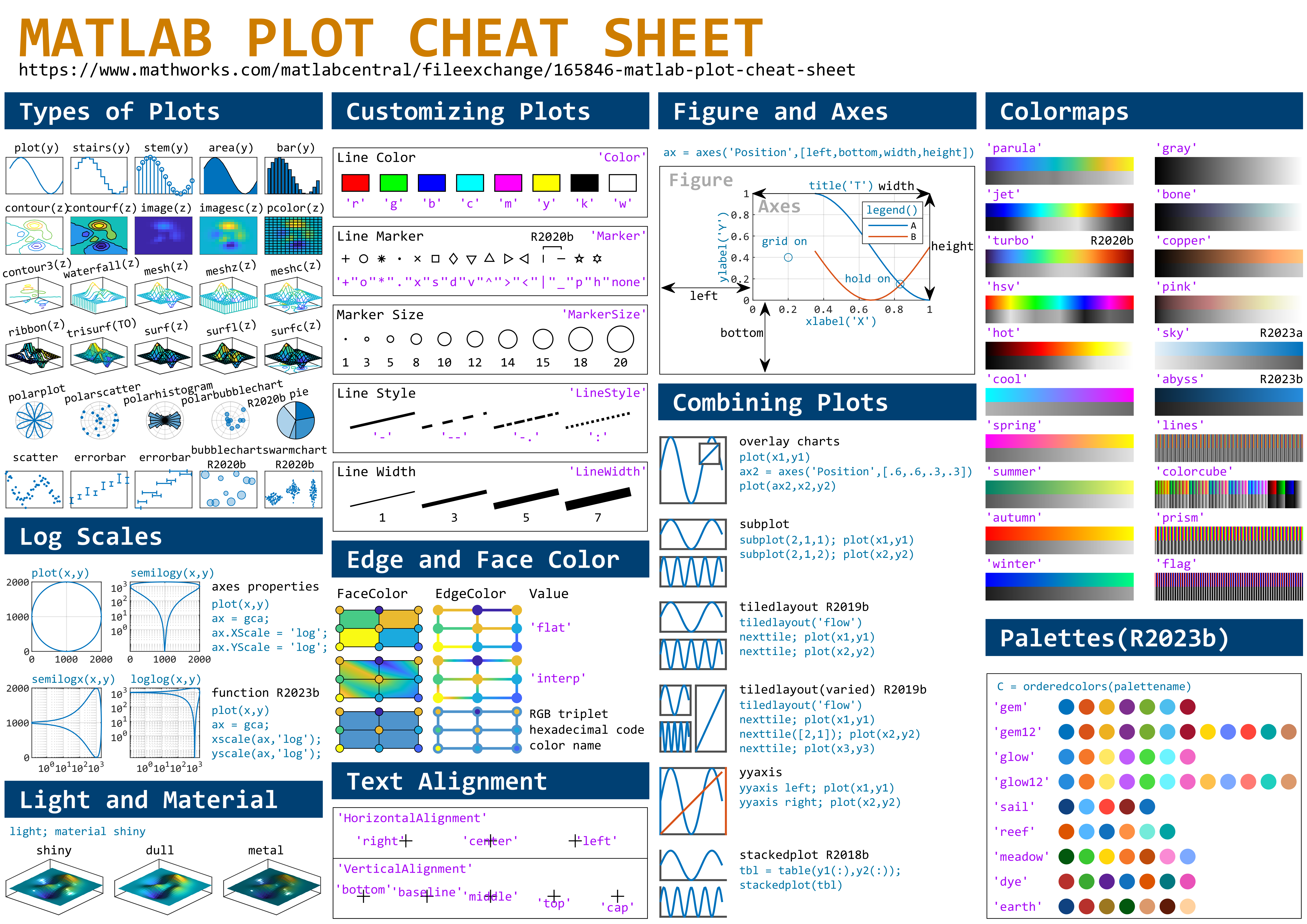
This cheat sheet is here:
reference:
- https://github.com/peijin94/matlabPlotCheatsheet
- https://github.com/mathworks/visualization-cheat-sheet
- https://www.mathworks.com/products/matlab/plot-gallery.html
- https://www.mathworks.com/help/matlab/release-notes.html
MATLAB used to have official visualization-cheat-sheet, but there have been quite a few new updates in MATLAB versions recently. Therefore, I made my own cheat sheet and marked the versions of each new thing that were released :
Dear MATLAB contest enthusiasts,
I believe many of you have been captivated by the innovative entries from Zhaoxu Liu / slanderer, in the 2023 MATLAB Flipbook Mini Hack contest.
Ever wondered about the person behind these creative entries? What drives a MATLAB user to such levels of skill? And what inspired his participation in the contest? We were just as curious as you are!
We were delighted to catch up with him and learn more about his use of MATLAB. The interview has recently been published in MathWorks Blogs. For an in-depth look into his insights and experiences, be sure to read our latest blog post: Community Q&A – Zhaoxu Liu.
But the conversation doesn't end here! Who would you like to see featured in our next interview? Drop their name in the comments section below and let us know who we should reach out to next!
Updating some of my educational Livescripts to 2024a, really love the new "define a function anywhere" feature, and have a "new" idea for improving Livescripts -- support "hidden" code blocks similar to the Jupyter Notebooks functionality.
For example, I often create "complicated" plots with a bunch of ancillary items and I don't want this code exposed to the reader by default, as it might confuse the reader. For example, consider a Livescript that might read like this:
-----
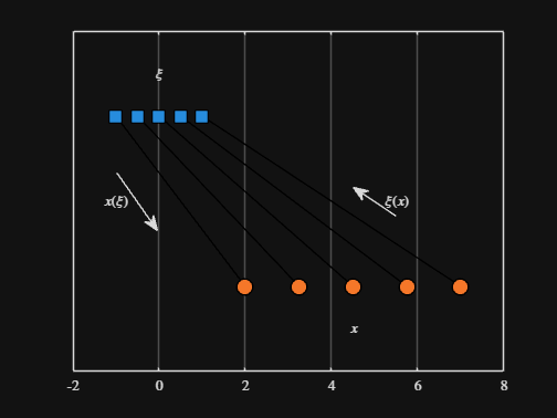
Noting the similar structure of these two mappings, let's now write a function that simply maps from some domain to some other domain using change of variable.
function x = ChangeOfVariable( x, from_domain, to_domain )
x = x - from_domain(1);
x = x * ( ( to_domain(2) - to_domain(1) ) / ( from_domain(2) - from_domain(1) ) );
x = x + to_domain(1);
end
Let's see this function in action
% HIDE CELL
clear
close all
from_domain = [-1, 1];
to_domain = [2, 7];
from_values = [-1, -0.5, 0, 0.5, 1];
to_values = ChangeOfVariable( from_values, from_domain, to_domain )
to_values = 1×5
2.0000 3.2500 4.5000 5.7500 7.0000
We can plot the values of from_values and to_values, showing how they're connected to each other:
% HIDE CELL
figure
hold on
for n = 1 : 5
plot( [from_values(n) to_values(n)], [1 0], Color="k", LineWidth=1 )
end
ax = gca;
ax.YTick = [];
ax.XLim = [ min( [from_domain, to_domain] ) - 1, max( [from_domain, to_domain] ) + 1 ];
ax.YLim = [-0.5, 1.5];
ax.XGrid = "on";
scatter( from_values, ones( 5, 1 ), Marker="s", MarkerFaceColor="flat", MarkerEdgeColor="k", SizeData=120, LineWidth=1, SeriesIndex=1 )
text( mean( from_domain ), 1.25, "$\xi$", Interpreter="latex", HorizontalAlignment="center", VerticalAlignment="middle" )
scatter( to_values, zeros( 5, 1 ), Marker="o", MarkerFaceColor="flat", MarkerEdgeColor="k", SizeData=120, LineWidth=1, SeriesIndex=2 )
text( mean( to_domain ), -0.25, "$x$", Interpreter="latex", HorizontalAlignment="center", VerticalAlignment="middle" )
scaled_arrow( ax, [mean( [from_domain(1), to_domain(1) ] ) - 1, 0.5], ( 1 - 0 ) / ( from_domain(1) - to_domain(1) ), 1 )
scaled_arrow( ax, [mean( [from_domain(end), to_domain(end)] ) + 1, 0.5], ( 1 - 0 ) / ( from_domain(end) - to_domain(end) ), -1 )
text( mean( [from_domain(1), to_domain(1) ] ) - 1.5, 0.5, "$x(\xi)$", Interpreter="latex", HorizontalAlignment="center", VerticalAlignment="middle" )
text( mean( [from_domain(end), to_domain(end)] ) + 1.5, 0.5, "$\xi(x)$", Interpreter="latex", HorizontalAlignment="center", VerticalAlignment="middle" )
-----
Where scaled_arrow is some utility function I've defined elsewhere... See how a majority of the code is simply "drivel" to create the plot, clear and close? I'd like to be able to hide those cells so that it would look more like this:
-----
Noting the similar structure of these two mappings, let's now write a function that simply maps from some domain to some other domain using change of variable.
function x = ChangeOfVariable( x, from_domain, to_domain )
x = x - from_domain(1);
x = x * ( ( to_domain(2) - to_domain(1) ) / ( from_domain(2) - from_domain(1) ) );
x = x + to_domain(1);
end
Let's see this function in action
▶ Show code cell
from_domain = [-1, 1];
to_domain = [2, 7];
from_values = [-1, -0.5, 0, 0.5, 1];
to_values = ChangeOfVariable( from_values, from_domain, to_domain )
to_values = 1×5
2.0000 3.2500 4.5000 5.7500 7.0000
We can plot the values of from_values and to_values, showing how they're connected to each other:
▶ Show code cell

-----
Thoughts?
I recently had issues with code folding seeming to disappear and it turns out that I had unknowingly disabled the "show code folding margin" option by accident. Despite using MATLAB for several years, I had no idea this was an option, especially since there seemed to be no references to it in the code folding part of the "Preferences" menu.
It would be great if in the future, there was a warning that told you about this when you try enable/disable folding in the Preferences.
I am using 2023b by the way.
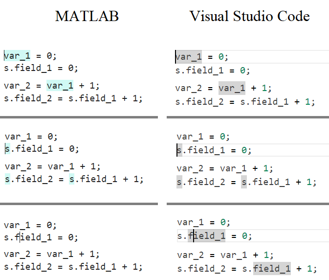
In the MATLAB editor, when clicking on a variable name, all the other instances of the variable name will be highlighted.
But this does not work for structure fields, which is a pity. Such feature would be quite often useful for me.
I show an illustration below, and compare it with Visual Studio Code that does it. ;-)
I am using MATLAB R2023a, sorry if it has been added to newer versions, but I didn't see it in the release notes.
Dear members, I’m currently doing research on the subject of using Generative A.I. as a digital designer. What our research group would like to know is which ethical issues have a big impact on the decisions you guys and girls make using generative A.I.
Whether you’re using A.I. or not, we would really like to know your vision and opinion about this subject. Please empty your thoughts and oppinion into your answers, we would like to get as much information as possible.
Are you currently using A.I. when doing your job? Yes, what for. No (not yet), why not?
Using A.I., would you use real information or alter names/numbers to get an answer?
What information would or wouldn’t you use? If the client is asking/ordering you to do certain things that go against your principles, would you still do it because order is order? How far would you go?
Who is responsible for the outcome of the generated content, you or the client?
Would you still feel like a product owner if it was co-developed with A.I.?
What we are looking for is that we would like to know why people do or don’t use AI in the field of design and wich ethical considerations they make. We’re just looking for general moral line of people, for example: 70% of designers don’t feel owner of a design that is generated by AI but 95% feels owner when it is co-created.
So therefore the questions we asked, we want to know the how you feel about this.
Temporary print statements are often helpful during debugging but it's easy to forget to remove the statements or sometimes you may not have writing privileges for the file. This tip uses conditional breakpoints to add print statements without ever editing the file!
What are conditional breakpoints?
Conditional breakpoints allow you to write a conditional statement that is executed when the selected line is hit and if the condition returns true, MATLAB pauses at that line. Otherwise, it continues.
The Hack: use ~fprintf() as the condition
fprintf prints information to the command window and returns the size of the message in bytes. The message size will always be greater than 0 which will always evaluate as true when converted to logical. Therefore, by negating an fprintf statement within a conditional breakpoint, the fprintf command will execute, print to the command window, and evalute as false which means the execution will continue uninterupted!
How to set a conditional break point
1. Right click the line number where you want the condition to be evaluated and select "Set Conditional Breakpoint"
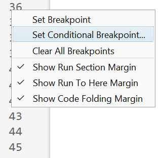
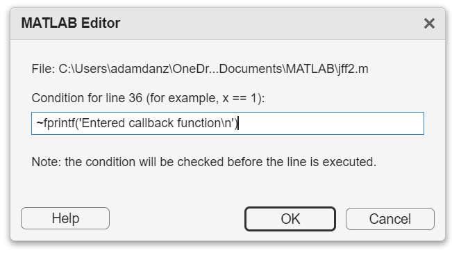
2. Enter a valid MATLAB expression that returns a logical scalar value in the editor dialog.
Handy one-liners
Check if a line is reached: Don't forget the negation (~) and the line break (\n)!
~fprintf('Entered callback function\n')
Display the call stack from the break point line: one of my favorites!
~fprintf('%s\n',formattedDisplayText(struct2table(dbstack)))
Inspect variable values: For scalar values,
~fprintf('v = %.5f\n', v)
~fprintf('%s\n', formattedDisplayText(v)).
Make sense of frequent hits: In some situations such as responses to listeners or interactive callbacks, a line can be executed 100s of times per second. Incorporate a timestamp to differentiate messages during rapid execution.
~fprintf('WindowButtonDownFcn - %s\n', datetime('now'))
Closing
This tip not only keeps your code clean but also offers a dynamic way to monitor code execution and variable states without permanent modifications. Interested in digging deeper? @Steve Eddins takes this tip to the next level with his Code Trace for MATLAB tool available on the File Exchange (read more).
Summary animation
To reproduce the events in this animation:
% buttonDownFcnDemo.m
fig = figure();
tcl = tiledlayout(4,4,'TileSpacing','compact');
for i = 1:16
ax = nexttile(tcl);
title(ax,"#"+string(i))
ax.ButtonDownFcn = @axesButtonDownFcn;
xlim(ax,[-1 1])
ylim(ax,[-1,1])
hold(ax,'on')
end
function axesButtonDownFcn(obj,event)
colors = lines(16);
plot(obj,event.IntersectionPoint(1),event.IntersectionPoint(2),...
'ko','MarkerFaceColor',colors(obj.Layout.Tile,:))
end
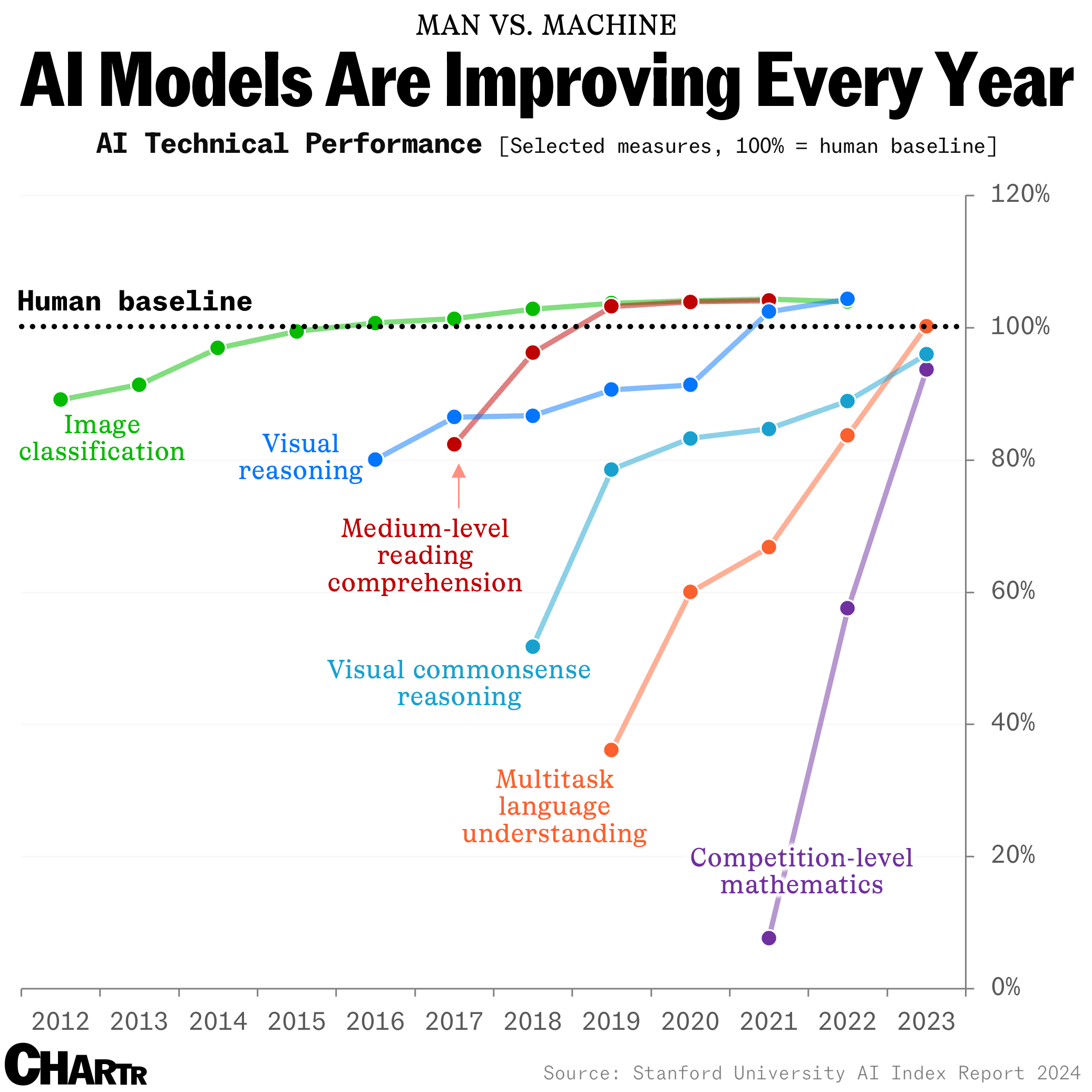
How long until the 'dumbest' models are smarter than your average person? Thanks for sharing this article @Adam Danz
The beautiful and elegant chord diagrams were all created using MATLAB?
Indeed, they were all generated using the chord diagram plotting toolkit that I developed myself:
- - Chord chart: [chord chart](https://www.mathworks.com/matlabcentral/fileexchange/116550-chord-chart)
- - Directed graph chord chart: [digraph chord chart]:(https://www.mathworks.com/matlabcentral/fileexchange/121043-digraph-chord-chart)
You can download these toolkits from the provided links.
The reason for writing this article is that many people have started using the chord diagram plotting toolkit that I developed. However, some users are unsure about customizing certain styles. As the developer, I have a good understanding of the implementation principles of the toolkit and can apply it flexibly. This has sparked the idea of challenging myself to create various styles of chord diagrams. Currently, the existing code is quite lengthy. In the future, I may integrate some of this code into the toolkit, enabling users to achieve the effects of many lines of code with just a few lines.
Without further ado, let's see the extent to which this MATLAB toolkit can currently perform.
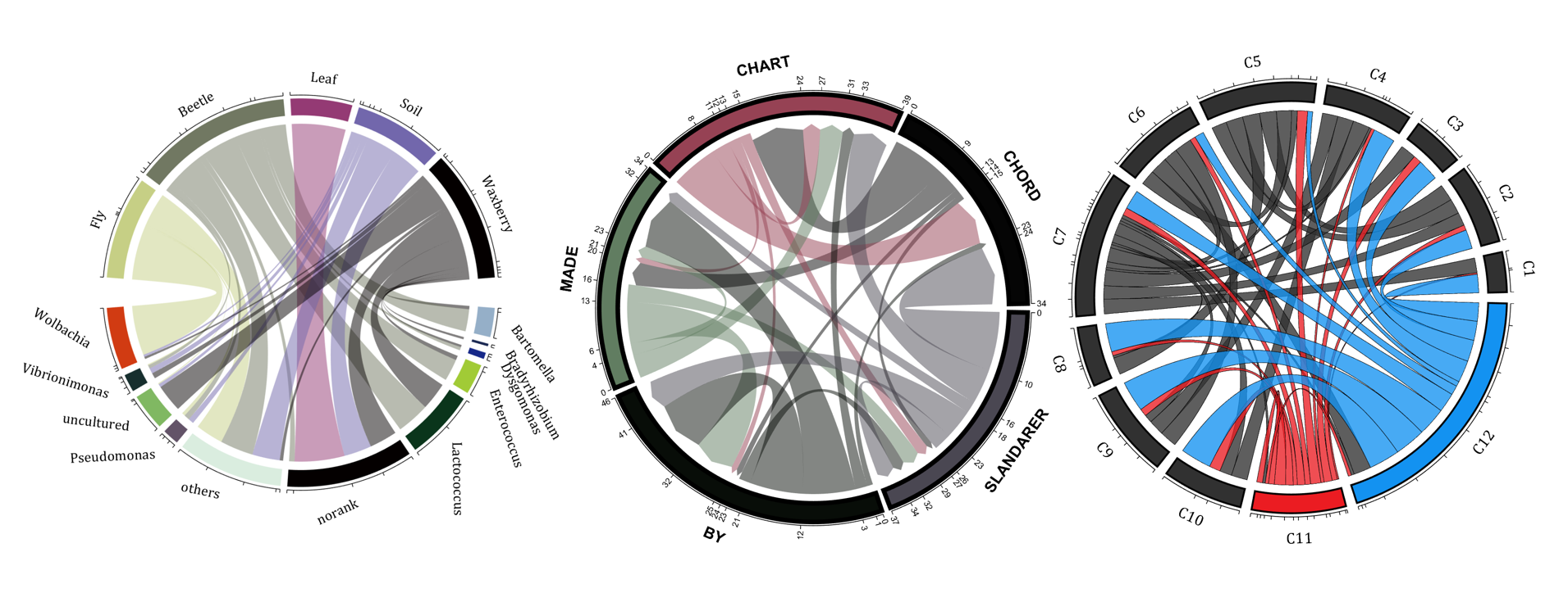
demo 1
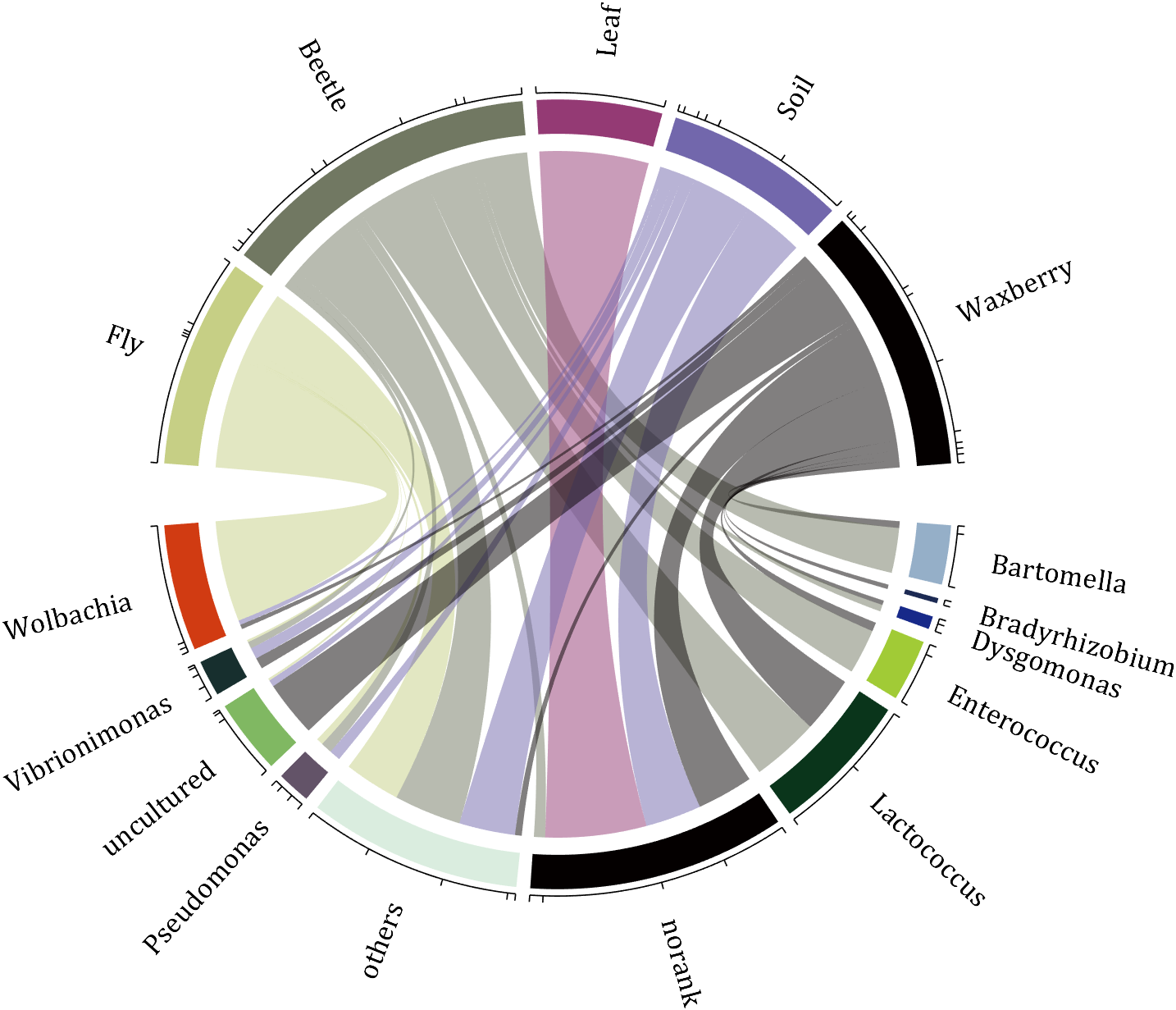
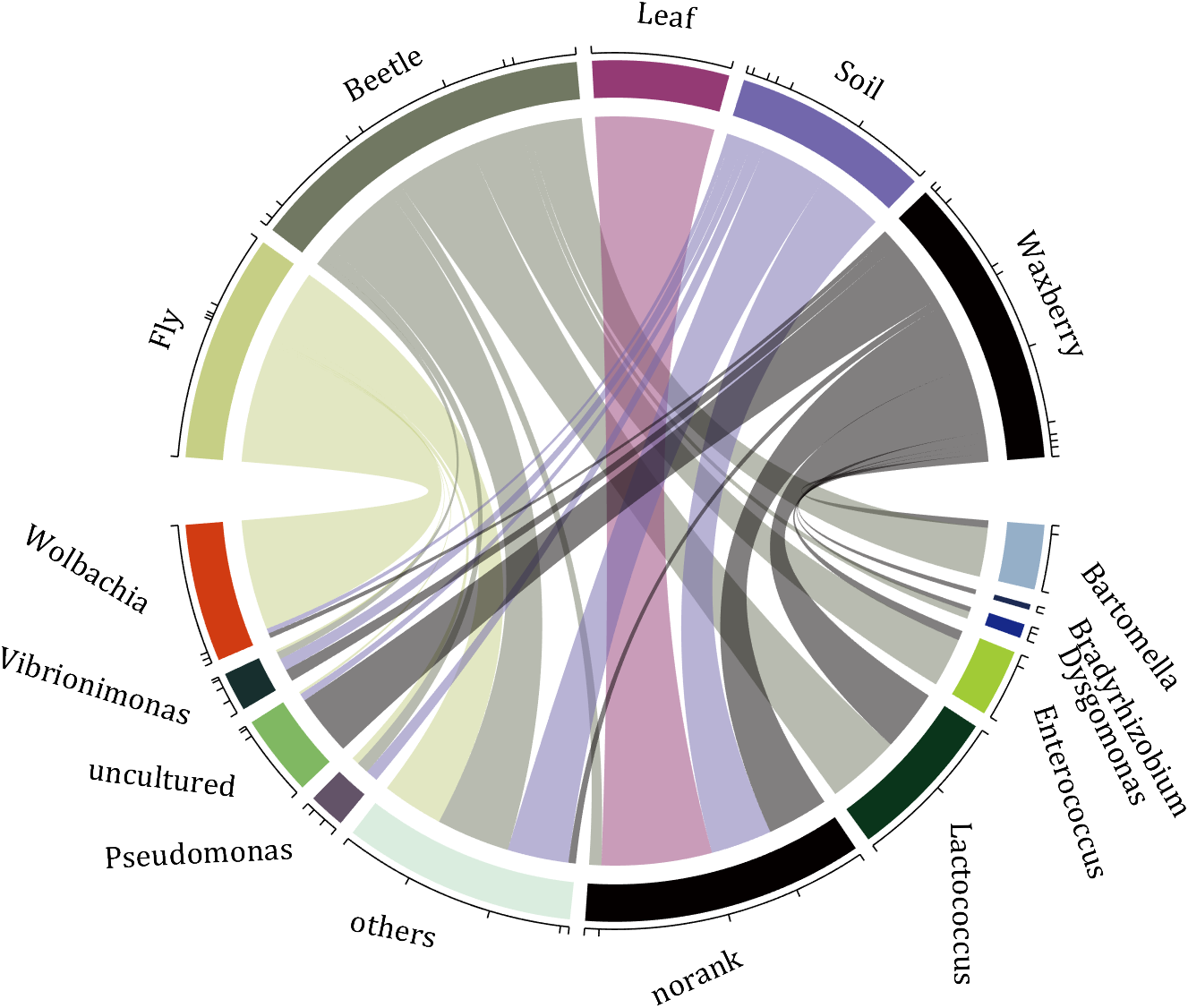
rng(2)
dataMat = randi([0,5], [11,5]);
dataMat(1:6,1) = 0;
dataMat([11,7],1) = [45,25];
dataMat([1,4,5,7],2) = [20,20,30,30];
dataMat(:,3) = 0;
dataMat(6,3) = 45;
dataMat(1:5,4) = 0;
dataMat([6,7],4) = [25,25];
dataMat([5,6,9],5) = [25,25,25];
colName = {'Fly', 'Beetle', 'Leaf', 'Soil', 'Waxberry'};
rowName = {'Bartomella', 'Bradyrhizobium', 'Dysgomonas', 'Enterococcus',...
'Lactococcus', 'norank', 'others', 'Pseudomonas', 'uncultured',...
'Vibrionimonas', 'Wolbachia'};
figure('Units','normalized', 'Position',[.02,.05,.6,.85])
CC = chordChart(dataMat, 'rowName',rowName, 'colName',colName, 'Sep',1/80);
CC = CC.draw();
% 修改上方方块颜色(Modify the color of the blocks above)
CListT = [0.7765 0.8118 0.5216; 0.4431 0.4706 0.3843; 0.5804 0.2275 0.4549;
0.4471 0.4039 0.6745; 0.0157 0 0 ];
for i = 1:size(dataMat, 2)
CC.setSquareT_N(i, 'FaceColor',CListT(i,:))
end
% 修改下方方块颜色(Modify the color of the blocks below)
CListF = [0.5843 0.6863 0.7843; 0.1098 0.1647 0.3255; 0.0902 0.1608 0.5373;
0.6314 0.7961 0.2118; 0.0392 0.2078 0.1059; 0.0157 0 0 ;
0.8549 0.9294 0.8745; 0.3882 0.3255 0.4078; 0.5020 0.7216 0.3843;
0.0902 0.1843 0.1804; 0.8196 0.2314 0.0706];
for i = 1:size(dataMat, 1)
CC.setSquareF_N(i, 'FaceColor',CListF(i,:))
end
% 修改弦颜色(Modify chord color)
for i = 1:size(dataMat, 1)
for j = 1:size(dataMat, 2)
CC.setChordMN(i,j, 'FaceColor',CListT(j,:), 'FaceAlpha',.5)
end
end
CC.tickState('on')
CC.labelRotate('on')
CC.setFont('FontSize',17, 'FontName','Cambria')
% CC.labelRotate('off')
% textHdl = findobj(gca,'Tag','ChordLabel');
% for i = 1:length(textHdl)
% if textHdl(i).Position(2) < 0
% if abs(textHdl(i).Position(1)) > .7
% textHdl(i).Rotation = textHdl(i).Rotation + 45;
% textHdl(i).HorizontalAlignment = 'right';
% if textHdl(i).Rotation > 90
% textHdl(i).Rotation = textHdl(i).Rotation + 180;
% textHdl(i).HorizontalAlignment = 'left';
% end
% else
% textHdl(i).Rotation = textHdl(i).Rotation + 10;
% textHdl(i).HorizontalAlignment = 'right';
% end
% end
% end
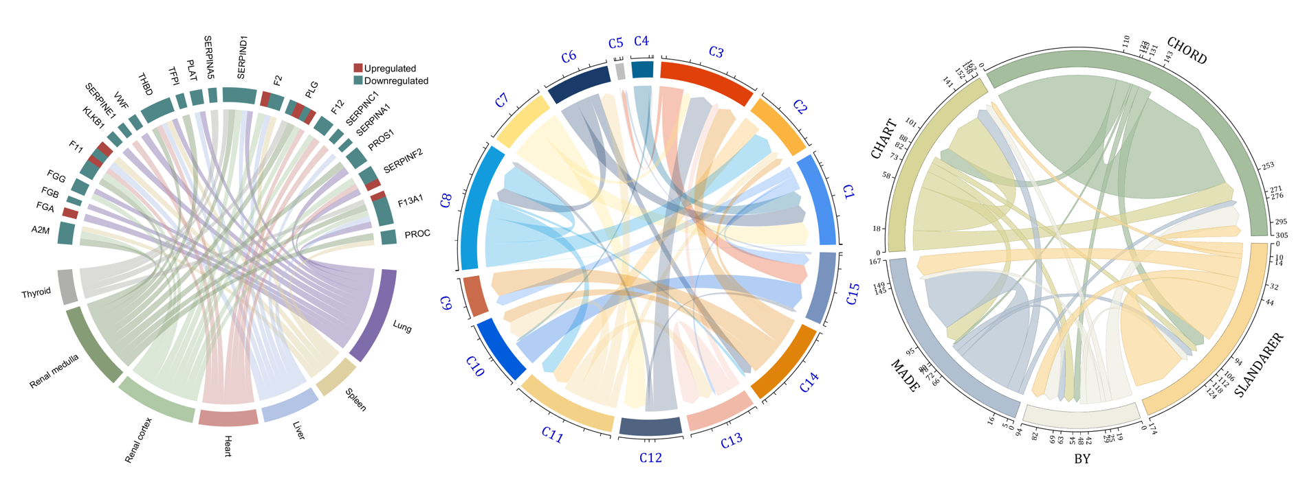
demo 2
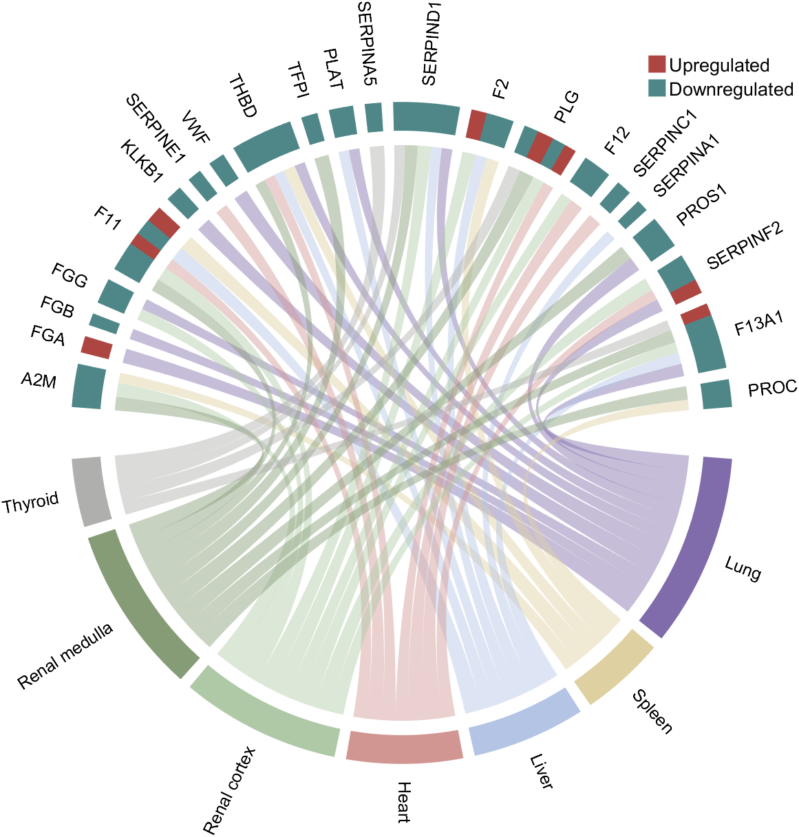
rng(3)
dataMat = randi([1,15], [7,22]);
dataMat(dataMat < 11) = 0;
dataMat(1, sum(dataMat, 1) == 0) = 15;
colName = {'A2M', 'FGA', 'FGB', 'FGG', 'F11', 'KLKB1', 'SERPINE1', 'VWF',...
'THBD', 'TFPI', 'PLAT', 'SERPINA5', 'SERPIND1', 'F2', 'PLG', 'F12',...
'SERPINC1', 'SERPINA1', 'PROS1', 'SERPINF2', 'F13A1', 'PROC'};
rowName = {'Lung', 'Spleen', 'Liver', 'Heart',...
'Renal cortex', 'Renal medulla', 'Thyroid'};
figure('Units','normalized', 'Position',[.02,.05,.6,.85])
CC = chordChart(dataMat, 'rowName',rowName, 'colName',colName, 'Sep',1/80, 'LRadius',1.21);
CC = CC.draw();
CC.labelRotate('on')
% 单独设置每一个弦末端方块(Set individual end blocks for each chord)
% Use obj.setEachSquareF_Prop
% or obj.setEachSquareT_Prop
% F means from (blocks below)
% T means to (blocks above)
CListT = [173,70,65; 79,135,136]./255;
% Upregulated:1 | Downregulated:2
Regulated = rand([7, 22]);
Regulated = (Regulated < .8) + 1;
for i = 1:size(Regulated, 1)
for j = 1:size(Regulated, 2)
CC.setEachSquareT_Prop(i, j, 'FaceColor', CListT(Regulated(i,j),:))
end
end
% 绘制图例(Draw legend)
H1 = fill([0,1,0] + 100, [1,0,1] + 100, CListT(1,:), 'EdgeColor','none');
H2 = fill([0,1,0] + 100, [1,0,1] + 100, CListT(2,:), 'EdgeColor','none');
lgdHdl = legend([H1,H2], {'Upregulated','Downregulated'}, 'AutoUpdate','off', 'Location','best');
lgdHdl.ItemTokenSize = [12,12];
lgdHdl.Box = 'off';
lgdHdl.FontSize = 13;
% 修改下方方块颜色(Modify the color of the blocks below)
CListF = [128,108,171; 222,208,161; 180,196,229; 209,150,146; 175,201,166;
134,156,118; 175,175,173]./255;
for i = 1:size(dataMat, 1)
CC.setSquareF_N(i, 'FaceColor',CListF(i,:))
end
% 修改弦颜色(Modify chord color)
for i = 1:size(dataMat, 1)
for j = 1:size(dataMat, 2)
CC.setChordMN(i,j, 'FaceColor',CListF(i,:), 'FaceAlpha',.45)
end
end
demo 3
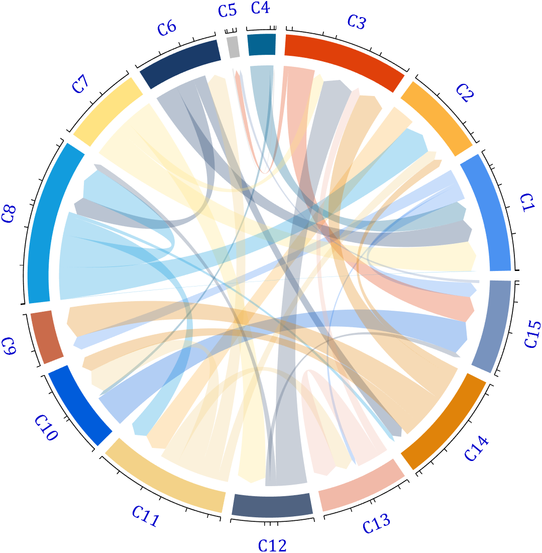
dataMat = rand([15,15]);
dataMat(dataMat > .15) = 0;
CList = [ 75,146,241; 252,180, 65; 224, 64, 10; 5,100,146; 191,191,191;
26, 59,105; 255,227,130; 18,156,221; 202,107, 75; 0, 92,219;
243,210,136; 80, 99,129; 241,185,168; 224,131, 10; 120,147,190]./255;
figure('Units','normalized', 'Position',[.02,.05,.6,.85])
BCC = biChordChart(dataMat, 'Arrow','on', 'CData',CList);
BCC = BCC.draw();
% 添加刻度
BCC.tickState('on')
% 修改字体,字号及颜色
BCC.setFont('FontName','Cambria', 'FontSize',17, 'Color',[0,0,.8])
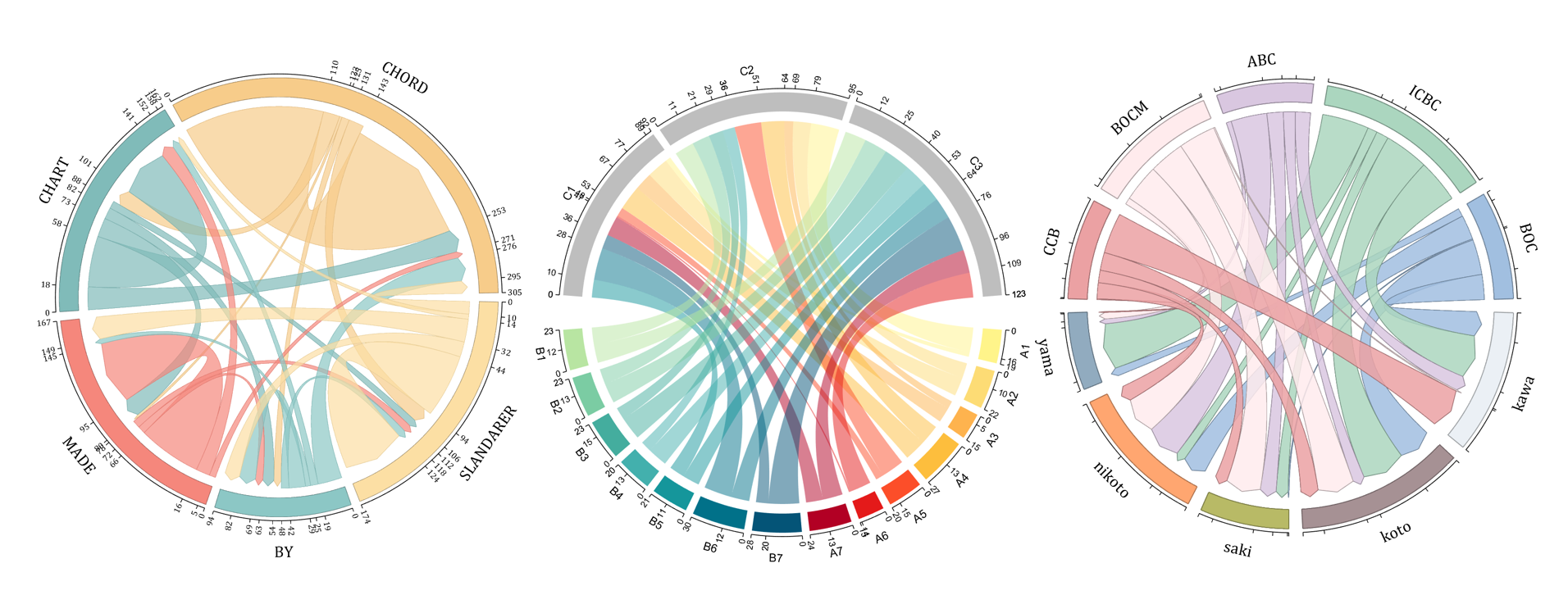
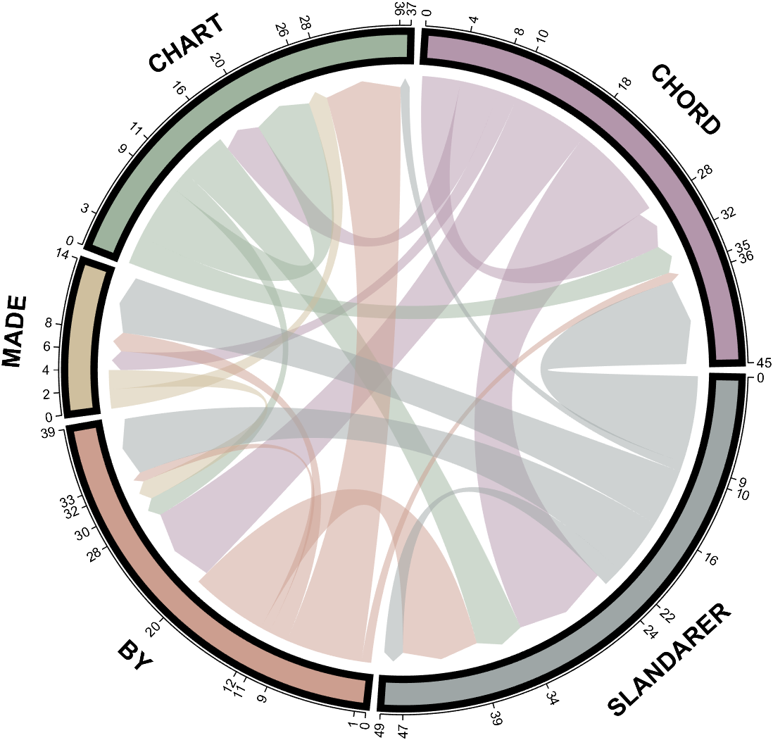
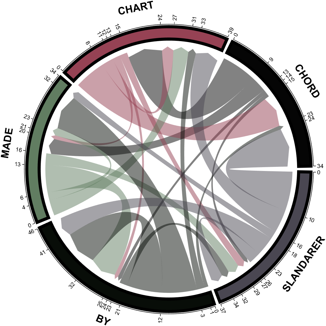
demo 4
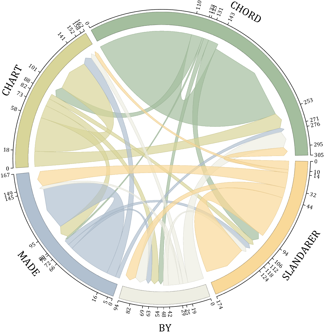
rng(5)
dataMat = randi([1,20], [5,5]);
dataMat(1,1) = 110;
dataMat(2,2) = 40;
dataMat(3,3) = 50;
dataMat(5,5) = 50;
CList1 = [164,190,158; 216,213,153; 177,192,208; 238,238,227; 249,217,153]./255;
CList2 = [247,204,138; 128,187,185; 245,135,124; 140,199,197; 252,223,164]./255;
CList = CList2;
NameList={'CHORD','CHART','MADE','BY','SLANDARER'};
figure('Units','normalized', 'Position',[.02,.05,.6,.85])
BCC = biChordChart(dataMat, 'Arrow','on', 'CData',CList, 'Sep',1/30, 'Label',NameList, 'LRadius',1.33);
BCC = BCC.draw();
% 添加刻度
BCC.tickState('on')
% 修改弦颜色(Modify chord color)
for i = 1:size(dataMat, 1)
for j = 1:size(dataMat, 2)
if dataMat(i,j) > 0
BCC.setChordMN(i,j, 'FaceAlpha',.7, 'EdgeColor',CList(i,:)./1.1)
end
end
end
% 修改方块颜色(Modify the color of the blocks)
for i = 1:size(dataMat, 1)
BCC.setSquareN(i, 'EdgeColor',CList(i,:)./1.7)
end
% 修改字体,字号及颜色
BCC.setFont('FontName','Cambria', 'FontSize',17)
BCC.tickLabelState('on')
BCC.setTickFont('FontName','Cambria', 'FontSize',9)
demo 5
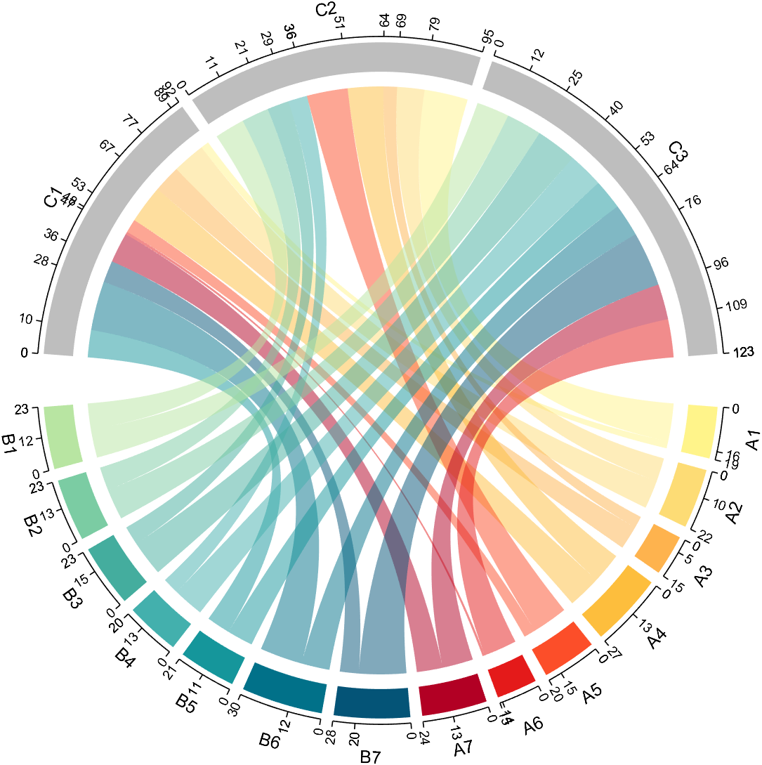
dataMat=randi([1,20], [14,3]);
dataMat(11:14,1) = 0;
dataMat(6:10,2) = 0;
dataMat(1:5,3) = 0;
colName = compose('C%d', 1:3);
rowName = [compose('A%d', 1:7), compose('B%d', 7:-1:1)];
figure('Units','normalized', 'Position',[.02,.05,.6,.85])
CC = chordChart(dataMat, 'rowName',rowName, 'colName',colName, 'Sep',1/80);
CC = CC.draw();
% 修改上方方块颜色(Modify the color of the blocks above)
for i = 1:size(dataMat, 2)
CC.setSquareT_N(i, 'FaceColor',[190,190,190]./255)
end
% 修改下方方块颜色(Modify the color of the blocks below)
CListF=[255,244,138; 253,220,117; 254,179, 78; 253,190, 61;
252, 78, 41; 228, 26, 26; 178, 0, 36; 4, 84,119;
1,113,137; 21,150,155; 67,176,173; 68,173,158;
123,204,163; 184,229,162]./255;
for i = 1:size(dataMat, 1)
CC.setSquareF_N(i, 'FaceColor',CListF(i,:))
end
% 修改弦颜色(Modify chord color)
for i = 1:size(dataMat, 1)
for j = 1:size(dataMat, 2)
CC.setChordMN(i,j, 'FaceColor',CListF(i,:), 'FaceAlpha',.5)
end
end
CC.tickState('on')
CC.tickLabelState('on')
demo 6
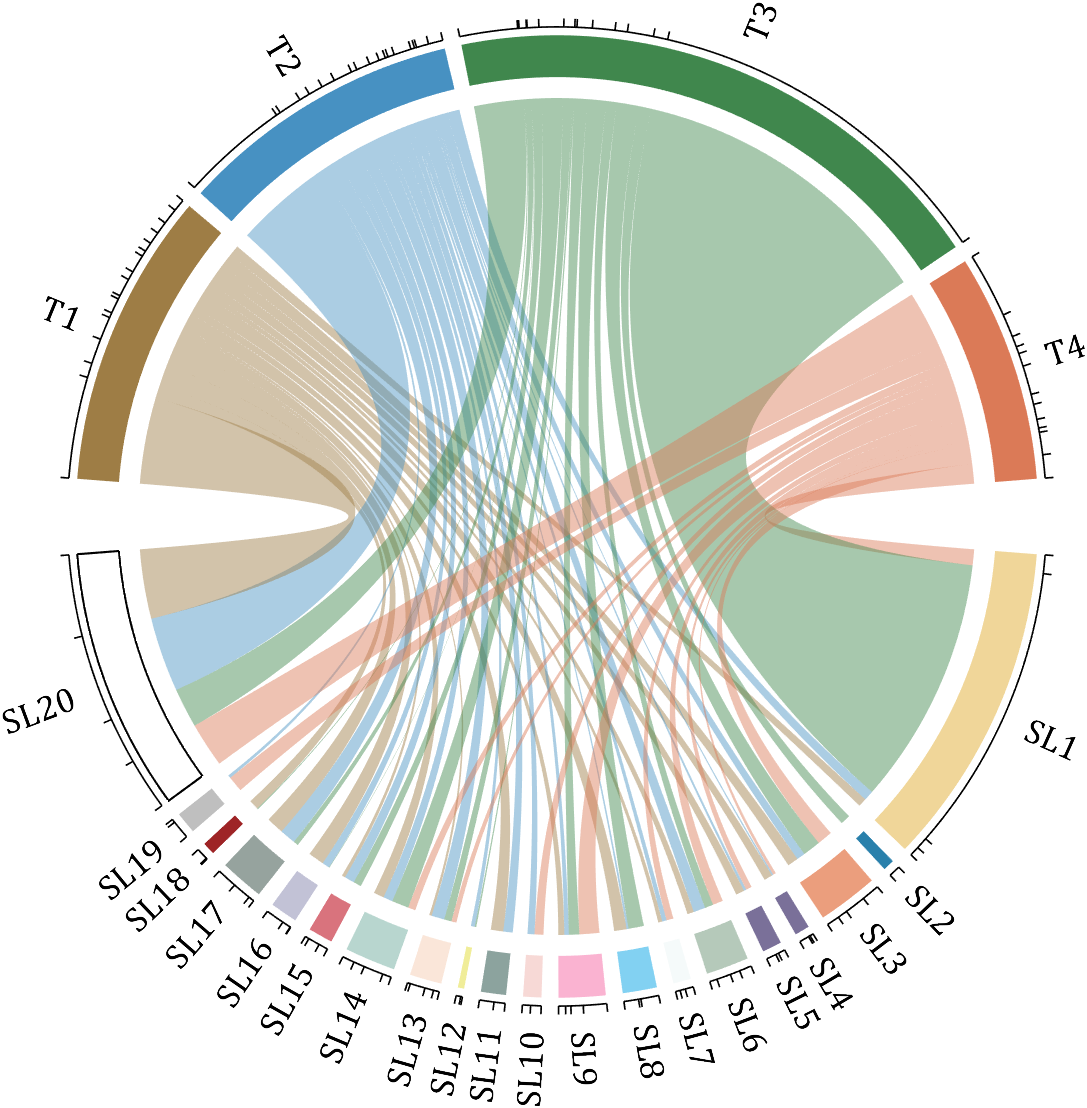
rng(2)
dataMat = randi([0,40], [20,4]);
dataMat(rand([20,4]) < .2) = 0;
dataMat(1,3) = 500;
dataMat(20,1:4) = [140; 150; 80; 90];
colName = compose('T%d', 1:4);
rowName = compose('SL%d', 1:20);
figure('Units','normalized', 'Position',[.02,.05,.6,.85])
CC = chordChart(dataMat, 'rowName',rowName, 'colName',colName, 'Sep',1/80, 'LRadius',1.23);
CC = CC.draw();
% 修改上方方块颜色(Modify the color of the blocks above)
CListT = [0.62,0.49,0.27; 0.28,0.57,0.76
0.25,0.53,0.30; 0.86,0.48,0.34];
for i = 1:size(dataMat, 2)
CC.setSquareT_N(i, 'FaceColor',CListT(i,:))
end
% 修改下方方块颜色(Modify the color of the blocks below)
CListF = [0.94,0.84,0.60; 0.16,0.50,0.67; 0.92,0.62,0.49;
0.48,0.44,0.60; 0.48,0.44,0.60; 0.71,0.79,0.73;
0.96,0.98,0.98; 0.51,0.82,0.95; 0.98,0.70,0.82;
0.97,0.85,0.84; 0.55,0.64,0.62; 0.94,0.93,0.60;
0.98,0.90,0.85; 0.72,0.84,0.81; 0.85,0.45,0.49;
0.76,0.76,0.84; 0.59,0.64,0.62; 0.62,0.14,0.15;
0.75,0.75,0.75; 1.00,1.00,1.00];
for i = 1:size(dataMat, 1)
CC.setSquareF_N(i, 'FaceColor',CListF(i,:))
end
CC.setSquareF_N(size(dataMat, 1), 'EdgeColor','k', 'LineWidth',1)
% 修改弦颜色(Modify chord color)
for i = 1:size(dataMat, 1)
for j = 1:size(dataMat, 2)
CC.setChordMN(i,j, 'FaceColor',CListT(j,:), 'FaceAlpha',.46)
end
end
CC.tickState('on')
CC.labelRotate('on')
CC.setFont('FontSize',17, 'FontName','Cambria')
demo 7
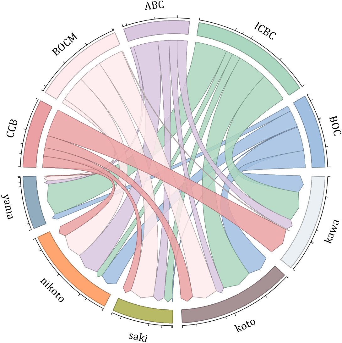
dataMat = randi([10,10000], [10,10]);
dataMat(6:10,:) = 0;
dataMat(:,1:5) = 0;
NameList = {'BOC', 'ICBC', 'ABC', 'BOCM', 'CCB', ...
'yama', 'nikoto', 'saki', 'koto', 'kawa'};
CList = [0.63,0.75,0.88
0.67,0.84,0.75
0.85,0.78,0.88
1.00,0.92,0.93
0.92,0.63,0.64
0.57,0.67,0.75
1.00,0.65,0.44
0.72,0.73,0.40
0.65,0.57,0.58
0.92,0.94,0.96];
figure('Units','normalized', 'Position',[.02,.05,.6,.85])
BCC = biChordChart(dataMat, 'Arrow','on', 'CData',CList, 'Label',NameList);
BCC = BCC.draw();
% 修改弦颜色(Modify chord color)
for i = 1:size(dataMat, 1)
for j = 1:size(dataMat, 2)
if dataMat(i,j) > 0
BCC.setChordMN(i,j, 'FaceAlpha',.85, 'EdgeColor',CList(i,:)./1.5, 'LineWidth',.8)
end
end
end
for i = 1:size(dataMat, 1)
BCC.setSquareN(i, 'EdgeColor',CList(i,:)./1.5, 'LineWidth',1)
end
% 添加刻度、修改字体
BCC.tickState('on')
BCC.setFont('FontName','Cambria', 'FontSize',17)
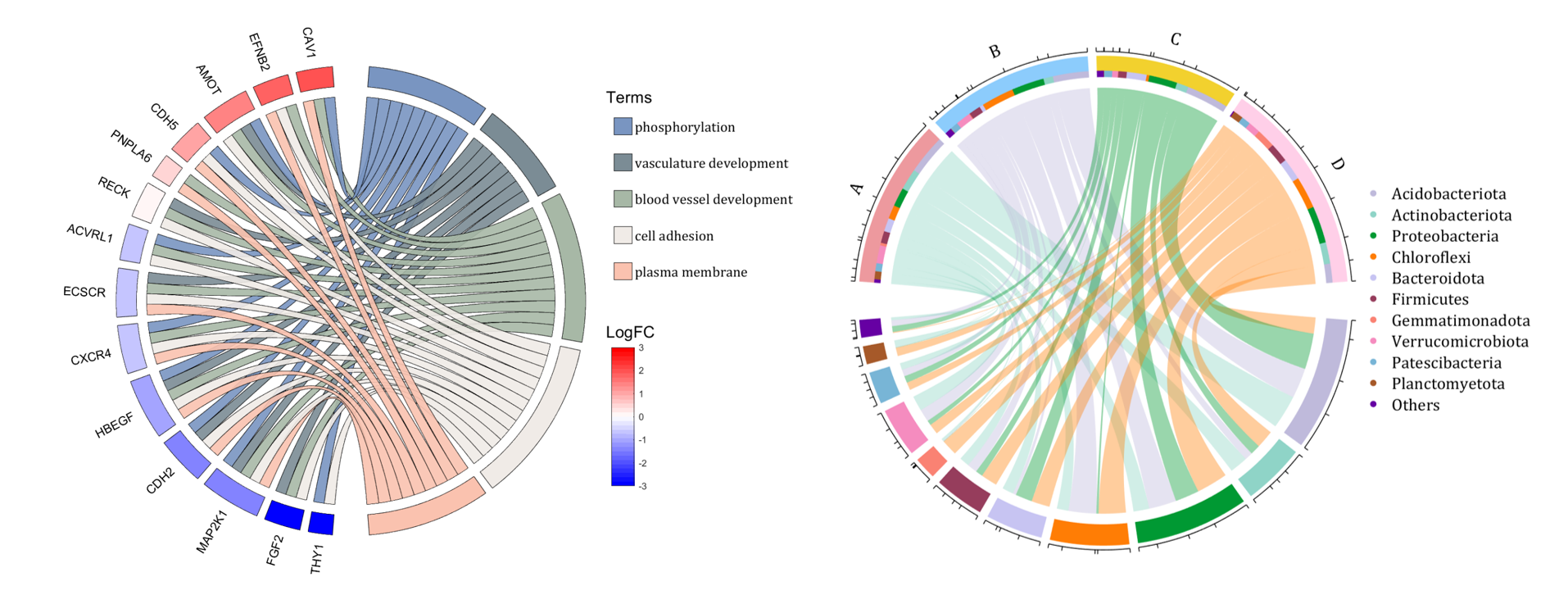
demo 8
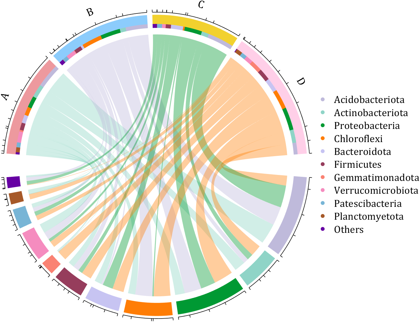
dataMat = rand([11,4]);
dataMat = round(10.*dataMat.*((11:-1:1).'+1))./10;
colName = {'A','B','C','D'};
rowName = {'Acidobacteriota', 'Actinobacteriota', 'Proteobacteria', ...
'Chloroflexi', 'Bacteroidota', 'Firmicutes', 'Gemmatimonadota', ...
'Verrucomicrobiota', 'Patescibacteria', 'Planctomyetota', 'Others'};
figure('Units','normalized', 'Position',[.02,.05,.8,.85])
CC = chordChart(dataMat, 'colName',colName, 'Sep',1/80, 'SSqRatio',30/100);% -30/100
CC = CC.draw();
% 修改上方方块颜色(Modify the color of the blocks above)
CListT = [0.93,0.60,0.62
0.55,0.80,0.99
0.95,0.82,0.18
1.00,0.81,0.91];
for i = 1:size(dataMat, 2)
CC.setSquareT_N(i, 'FaceColor',CListT(i,:))
end
% 修改下方方块颜色(Modify the color of the blocks below)
CListF = [0.75,0.73,0.86
0.56,0.83,0.78
0.00,0.60,0.20
1.00,0.49,0.02
0.78,0.77,0.95
0.59,0.24,0.36
0.98,0.51,0.45
0.96,0.55,0.75
0.47,0.71,0.84
0.65,0.35,0.16
0.40,0.00,0.64];
for i = 1:size(dataMat, 1)
CC.setSquareF_N(i, 'FaceColor',CListF(i,:))
end
% 修改弦颜色(Modify chord color)
CListC = [0.55,0.83,0.76
0.75,0.73,0.86
0.00,0.60,0.19
1.00,0.51,0.04];
for i = 1:size(dataMat, 1)
for j = 1:size(dataMat, 2)
CC.setChordMN(i,j, 'FaceColor',CListC(j,:), 'FaceAlpha',.4)
end
end
% 单独设置每一个弦末端方块(Set individual end blocks for each chord)
% Use obj.setEachSquareF_Prop
% or obj.setEachSquareT_Prop
% F means from (blocks below)
% T means to (blocks above)
for i = 1:size(dataMat, 1)
for j = 1:size(dataMat, 2)
CC.setEachSquareT_Prop(i,j, 'FaceColor', CListF(i,:))
end
end
% 添加刻度
CC.tickState('on')
% 修改字体,字号及颜色
CC.setFont('FontName','Cambria', 'FontSize',17)
% 隐藏下方标签
textHdl = findobj(gca, 'Tag','ChordLabel');
for i = 1:length(textHdl)
if textHdl(i).Position(2) < 0
set(textHdl(i), 'Visible','off')
end
end
% 绘制图例(Draw legend)
scatterHdl = scatter(10.*ones(size(dataMat,1)),10.*ones(size(dataMat,1)), ...
55, 'filled');
for i = 1:length(scatterHdl)
scatterHdl(i).CData = CListF(i,:);
end
lgdHdl = legend(scatterHdl, rowName, 'Location','best', 'FontSize',16, 'FontName','Cambria', 'Box','off');
set(lgdHdl, 'Position',[.7482,.3577,.1658,.3254])
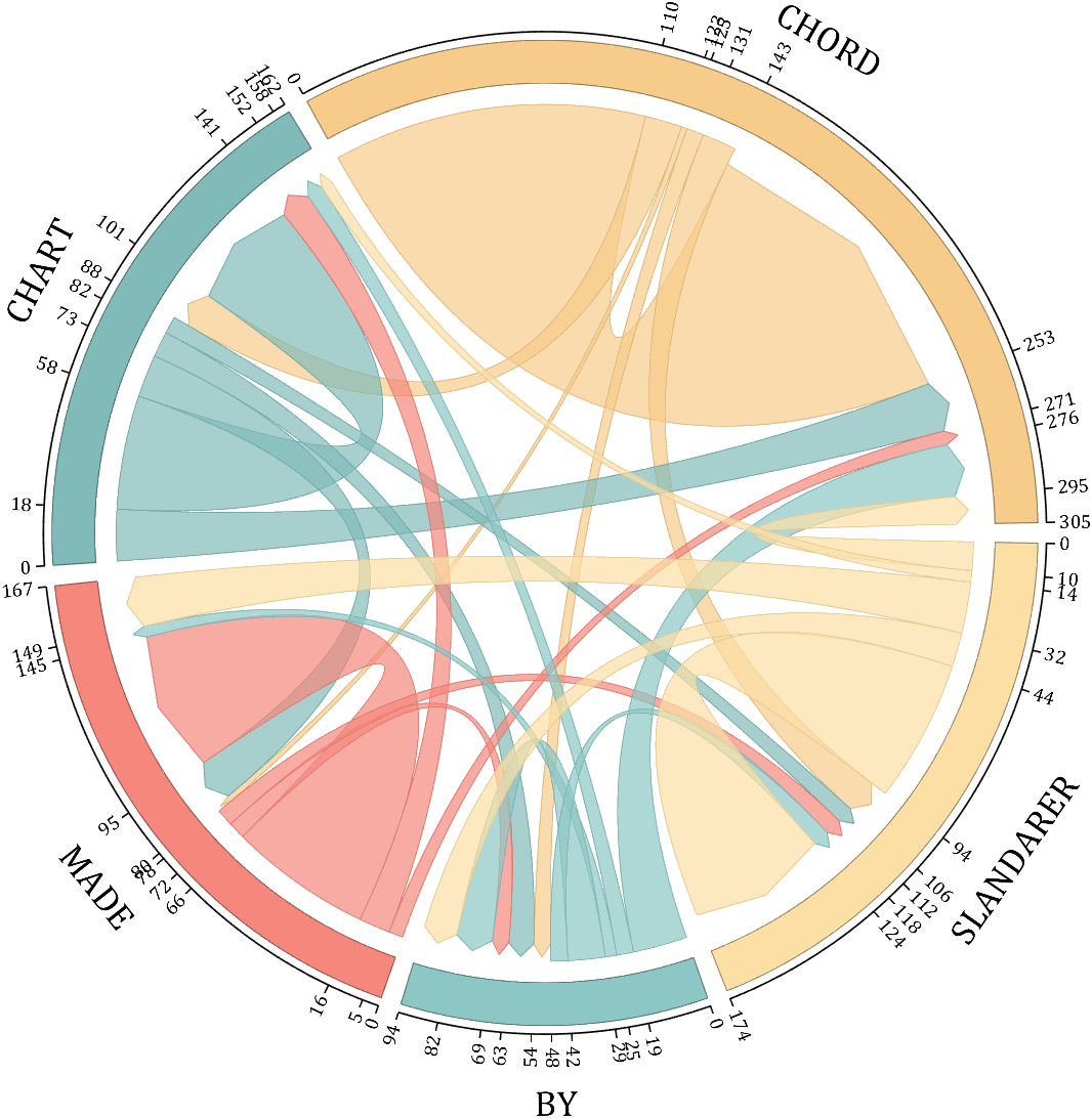
demo 9
dataMat = randi([0,10], [5,5]);
CList1 = [0.70,0.59,0.67
0.62,0.70,0.62
0.81,0.75,0.62
0.80,0.62,0.56
0.62,0.65,0.65];
CList2 = [0.02,0.02,0.02
0.59,0.26,0.33
0.38,0.49,0.38
0.03,0.05,0.03
0.29,0.28,0.32];
CList = CList2;
NameList={'CHORD','CHART','MADE','BY','SLANDARER'};
figure('Units','normalized', 'Position',[.02,.05,.6,.85])
BCC = biChordChart(dataMat, 'Arrow','on', 'CData',CList, 'Sep',1/30, 'Label',NameList, 'LRadius',1.33);
BCC = BCC.draw();
% 修改弦颜色(Modify chord color)
for i = 1:size(dataMat, 1)
for j = 1:size(dataMat, 2)
BCC.setChordMN(i,j, 'FaceAlpha',.5)
end
end
% 修改方块颜色(Modify the color of the blocks)
for i = 1:size(dataMat, 1)
BCC.setSquareN(i, 'EdgeColor',[0,0,0], 'LineWidth',5)
end
% 添加刻度
BCC.tickState('on')
% 修改字体,字号及颜色
BCC.setFont('FontSize',17, 'FontWeight','bold')
BCC.tickLabelState('on')
BCC.setTickFont('FontSize',9)
demo 10
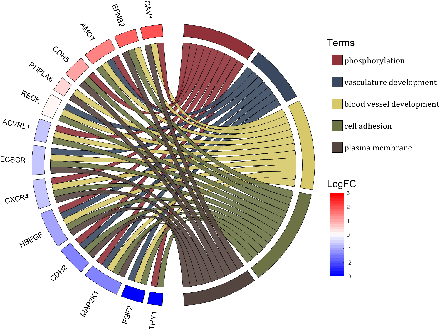
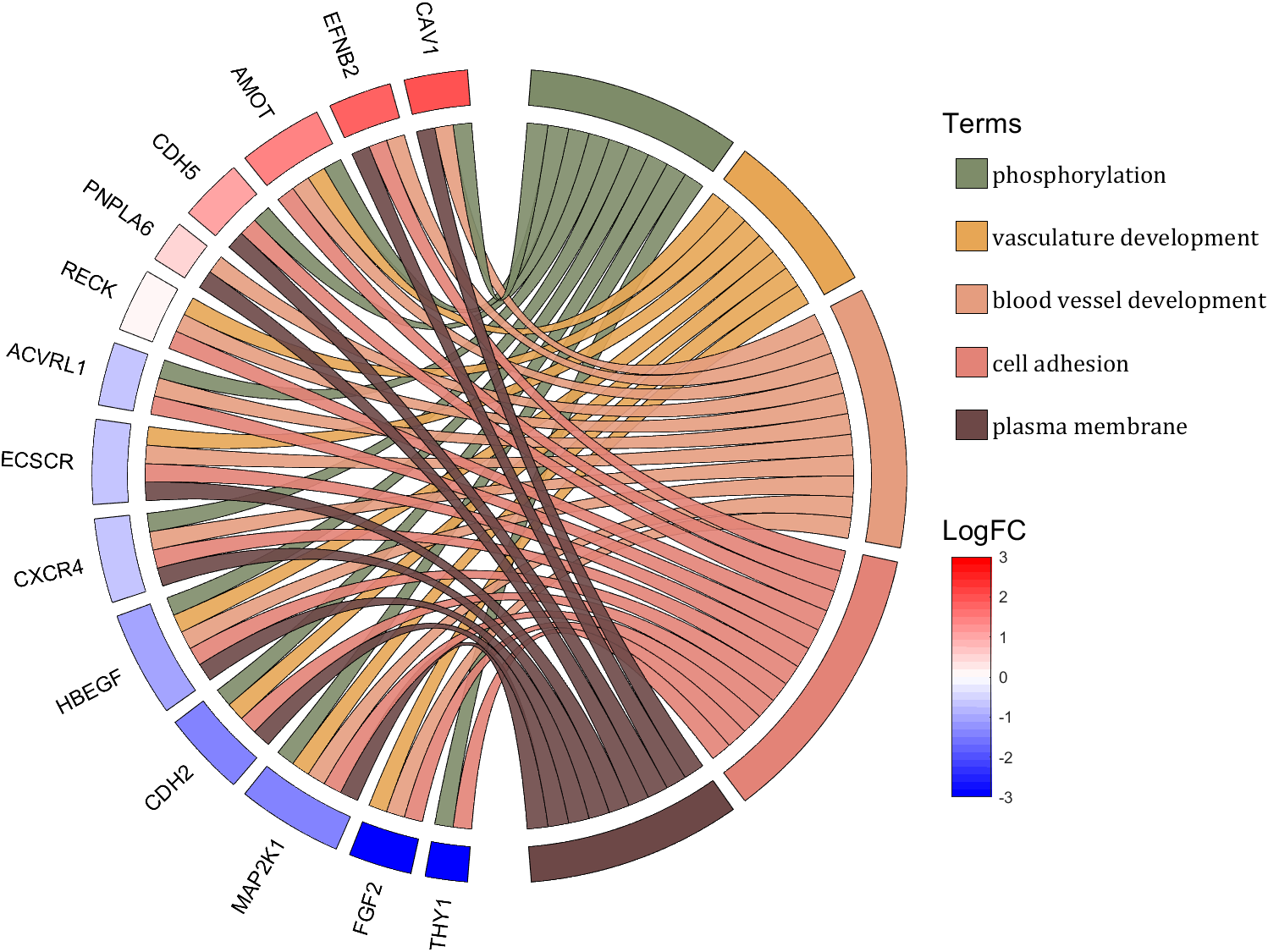
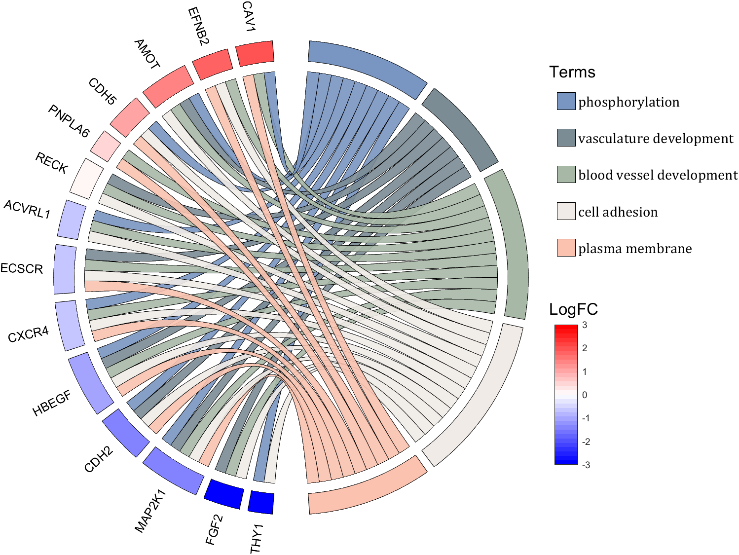
rng(2)
dataMat = rand([14,5]) > .3;
colName = {'phosphorylation', 'vasculature development', 'blood vessel development', ...
'cell adhesion', 'plasma membrane'};
rowName = {'THY1', 'FGF2', 'MAP2K1', 'CDH2', 'HBEGF', 'CXCR4', 'ECSCR',...
'ACVRL1', 'RECK', 'PNPLA6', 'CDH5', 'AMOT', 'EFNB2', 'CAV1'};
figure('Units','normalized', 'Position',[.02,.05,.9,.85])
CC = chordChart(dataMat, 'colName',colName, 'rowName',rowName, 'Sep',1/80, 'LRadius',1.2);
CC = CC.draw();
% 修改上方方块颜色(Modify the color of the blocks above)
CListT1 = [0.5686 0.1961 0.2275
0.2275 0.2863 0.3765
0.8431 0.7882 0.4118
0.4275 0.4510 0.2706
0.3333 0.2706 0.2510];
CListT2 = [0.4941 0.5490 0.4118
0.9059 0.6510 0.3333
0.8980 0.6157 0.4980
0.8902 0.5137 0.4667
0.4275 0.2824 0.2784];
CListT3 = [0.4745 0.5843 0.7569
0.4824 0.5490 0.5843
0.6549 0.7216 0.6510
0.9412 0.9216 0.9059
0.9804 0.7608 0.6863];
CListT = CListT3;
for i = 1:size(dataMat, 2)
CC.setSquareT_N(i, 'FaceColor',CListT(i,:), 'EdgeColor',[0,0,0])
end
% 修改弦颜色(Modify chord color)
for i = 1:size(dataMat, 1)
for j = 1:size(dataMat, 2)
CC.setChordMN(i,j, 'FaceColor',CListT(j,:), 'FaceAlpha',.9, 'EdgeColor',[0,0,0])
end
end
% 修改下方方块颜色(Modify the color of the blocks below)
logFC = sort(rand(1,14))*6 - 3;
for i = 1:size(dataMat, 1)
CC.setSquareF_N(i, 'CData',logFC(i), 'FaceColor','flat', 'EdgeColor',[0,0,0])
end
CMap = [ 0 0 1.0000; 0.0645 0.0645 1.0000; 0.1290 0.1290 1.0000; 0.1935 0.1935 1.0000
0.2581 0.2581 1.0000; 0.3226 0.3226 1.0000; 0.3871 0.3871 1.0000; 0.4516 0.4516 1.0000
0.5161 0.5161 1.0000; 0.5806 0.5806 1.0000; 0.6452 0.6452 1.0000; 0.7097 0.7097 1.0000
0.7742 0.7742 1.0000; 0.8387 0.8387 1.0000; 0.9032 0.9032 1.0000; 0.9677 0.9677 1.0000
1.0000 0.9677 0.9677; 1.0000 0.9032 0.9032; 1.0000 0.8387 0.8387; 1.0000 0.7742 0.7742
1.0000 0.7097 0.7097; 1.0000 0.6452 0.6452; 1.0000 0.5806 0.5806; 1.0000 0.5161 0.5161
1.0000 0.4516 0.4516; 1.0000 0.3871 0.3871; 1.0000 0.3226 0.3226; 1.0000 0.2581 0.2581
1.0000 0.1935 0.1935; 1.0000 0.1290 0.1290; 1.0000 0.0645 0.0645; 1.0000 0 0];
colormap(CMap);
try clim([-3,3]),catch,end
try caxis([-3,3]),catch,end
CBHdl = colorbar();
CBHdl.Position = [0.74,0.25,0.02,0.2];
% =========================================================================
% 交换XY轴(Swap XY axis)
patchHdl = findobj(gca, 'Type','patch');
for i = 1:length(patchHdl)
tX = patchHdl(i).XData;
tY = patchHdl(i).YData;
patchHdl(i).XData = tY;
patchHdl(i).YData = - tX;
end
txtHdl = findobj(gca, 'Type','text');
for i = 1:length(txtHdl)
txtHdl(i).Position([1,2]) = [1,-1].*txtHdl(i).Position([2,1]);
if txtHdl(i).Position(1) < 0
txtHdl(i).HorizontalAlignment = 'right';
else
txtHdl(i).HorizontalAlignment = 'left';
end
end
lineHdl = findobj(gca, 'Type','line');
for i = 1:length(lineHdl)
tX = lineHdl(i).XData;
tY = lineHdl(i).YData;
lineHdl(i).XData = tY;
lineHdl(i).YData = - tX;
end
% =========================================================================
txtHdl = findobj(gca, 'Type','text');
for i = 1:length(txtHdl)
if txtHdl(i).Position(1) > 0
txtHdl(i).Visible = 'off';
end
end
text(1.25,-.15, 'LogFC', 'FontSize',16)
text(1.25,1, 'Terms', 'FontSize',16)
patchHdl = [];
for i = 1:size(dataMat, 2)
patchHdl(i) = fill([10,11,12],[10,13,13], CListT(i,:), 'EdgeColor',[0,0,0]);
end
lgdHdl = legend(patchHdl, colName, 'Location','best', 'FontSize',14, 'FontName','Cambria', 'Box','off');
lgdHdl.Position = [.735,.53,.167,.27];
lgdHdl.ItemTokenSize = [18,8];
demo 11
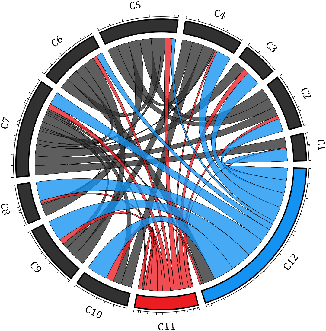
rng(2)
dataMat = rand([12,12]);
dataMat(dataMat < .85) = 0;
dataMat(7,:) = 1.*(rand(1,12)+.1);
dataMat(11,:) = .6.*(rand(1,12)+.1);
dataMat(12,:) = [2.*(rand(1,10)+.1), 0, 0];
CList = [repmat([49,49,49],[10,1]); 235,28,34; 19,146,241]./255;
figure('Units','normalized', 'Position',[.02,.05,.6,.85])
BCC = biChordChart(dataMat, 'Arrow','off', 'CData',CList);
BCC = BCC.draw();
% 添加刻度
BCC.tickState('on')
% 修改字体,字号及颜色
BCC.setFont('FontName','Cambria', 'FontSize',17)
% 修改弦颜色(Modify chord color)
for i = 1:size(dataMat, 1)
for j = 1:size(dataMat, 2)
if dataMat(i,j) > 0
BCC.setChordMN(i,j, 'FaceAlpha',.78, 'EdgeColor',[0,0,0])
end
end
end
% 修改方块颜色(Modify the color of the blocks)
for i = 1:size(dataMat, 1)
BCC.setSquareN(i, 'EdgeColor',[0,0,0], 'LineWidth',2)
end
demo 12
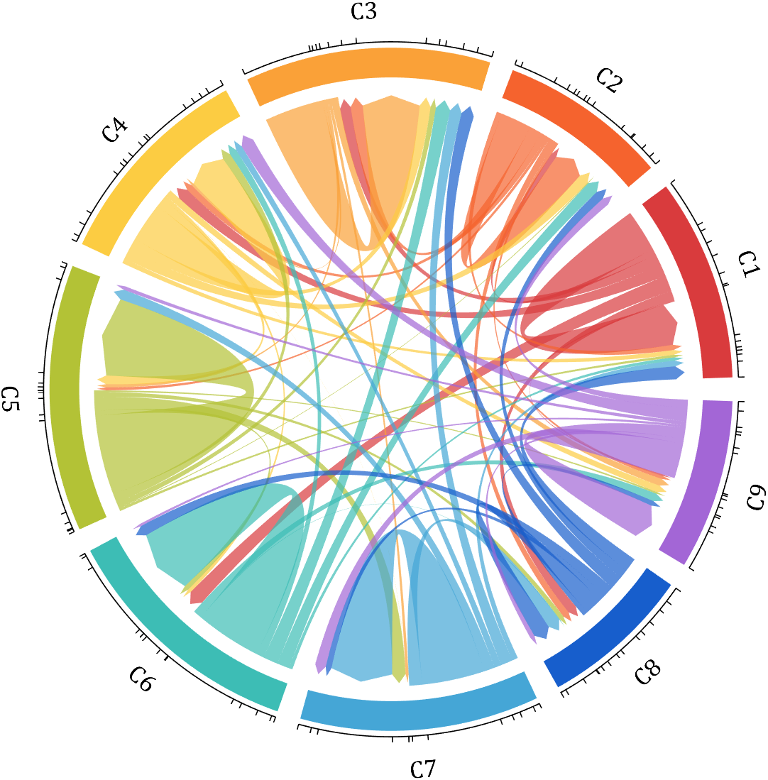
dataMat = rand([9,9]);
dataMat(dataMat > .7) = 0;
dataMat(eye(9) == 1) = (rand([1,9])+.2).*3;
CList = [0.85,0.23,0.24
0.96,0.39,0.18
0.98,0.63,0.22
0.99,0.80,0.26
0.70,0.76,0.21
0.24,0.74,0.71
0.27,0.65,0.84
0.09,0.37,0.80
0.64,0.40,0.84];
figure('Units','normalized', 'Position',[.02,.05,.6,.85])
BCC = biChordChart(dataMat, 'Arrow','on', 'CData',CList);
BCC = BCC.draw();
% 添加刻度、刻度标签
BCC.tickState('on')
% 修改字体,字号及颜色
BCC.setFont('FontName','Cambria', 'FontSize',17)
% 修改弦颜色(Modify chord color)
for i = 1:size(dataMat, 1)
for j = 1:size(dataMat, 2)
if dataMat(i,j) > 0
BCC.setChordMN(i,j, 'FaceAlpha',.7)
end
end
end
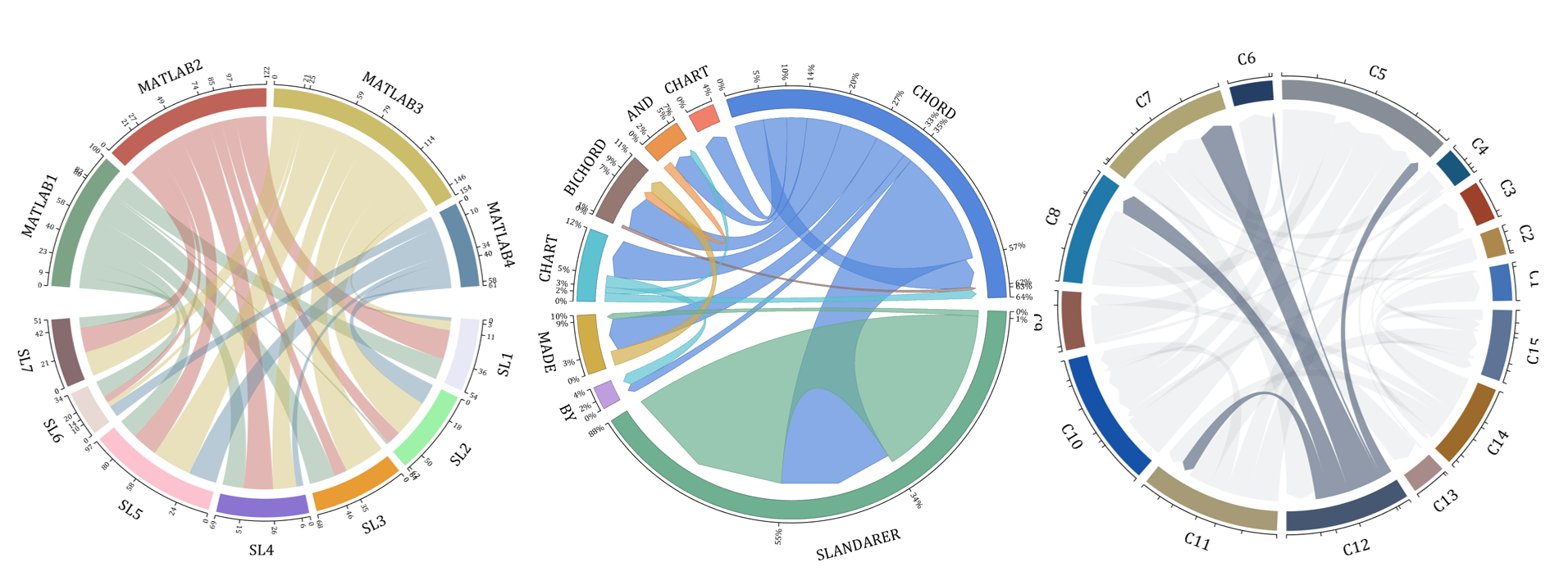
demo 13
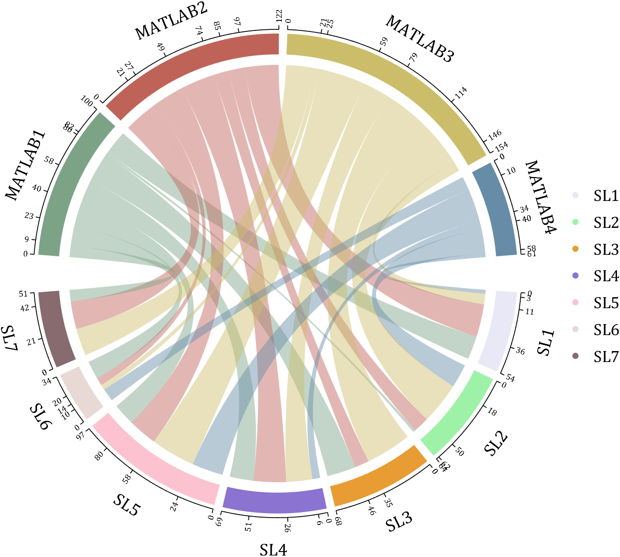
rng(2)
dataMat = randi([1,40], [7,4]);
dataMat(rand([7,4]) < .1) = 0;
colName = compose('MATLAB%d', 1:4);
rowName = compose('SL%d', 1:7);
figure('Units','normalized', 'Position',[.02,.05,.7,.85])
CC = chordChart(dataMat, 'rowName',rowName, 'colName',colName, 'Sep',1/80, 'LRadius',1.32);
CC = CC.draw();
% 修改上方方块颜色(Modify the color of the blocks above)
CListT = [0.49,0.64,0.53
0.75,0.39,0.35
0.80,0.74,0.42
0.40,0.55,0.66];
for i = 1:size(dataMat, 2)
CC.setSquareT_N(i, 'FaceColor',CListT(i,:))
end
% 修改下方方块颜色(Modify the color of the blocks below)
CListF = [0.91,0.91,0.97
0.62,0.95,0.66
0.91,0.61,0.20
0.54,0.45,0.82
0.99,0.76,0.81
0.91,0.85,0.83
0.53,0.42,0.43];
for i = 1:size(dataMat, 1)
CC.setSquareF_N(i, 'FaceColor',CListF(i,:))
end
% 修改弦颜色(Modify chord color)
for i = 1:size(dataMat, 1)
for j = 1:size(dataMat, 2)
CC.setChordMN(i,j, 'FaceColor',CListT(j,:), 'FaceAlpha',.46)
end
end
CC.tickState('on')
CC.tickLabelState('on')
CC.setFont('FontSize',17, 'FontName','Cambria')
CC.setTickFont('FontSize',8, 'FontName','Cambria')
% 绘制图例(Draw legend)
scatterHdl = scatter(10.*ones(size(dataMat,1)),10.*ones(size(dataMat,1)), ...
55, 'filled');
for i = 1:length(scatterHdl)
scatterHdl(i).CData = CListF(i,:);
end
lgdHdl = legend(scatterHdl, rowName, 'Location','best', 'FontSize',16, 'FontName','Cambria', 'Box','off');
set(lgdHdl, 'Position',[.77,.38,.1658,.27])
demo 14
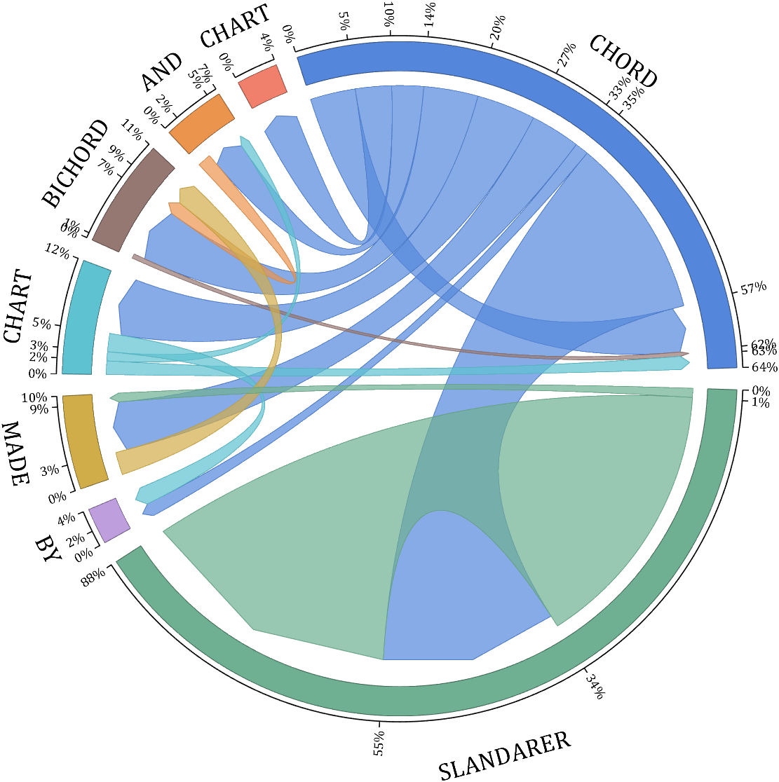
rng(6)
dataMat = randi([1,20], [8,8]);
dataMat(dataMat > 5) = 0;
dataMat(1,:) = randi([1,15], [1,8]);
dataMat(1,8) = 40;
dataMat(8,8) = 60;
dataMat = dataMat./sum(sum(dataMat));
CList = [0.33,0.53,0.86
0.94,0.50,0.42
0.92,0.58,0.30
0.59,0.47,0.45
0.37,0.76,0.82
0.82,0.68,0.29
0.75,0.62,0.87
0.43,0.69,0.57];
NameList={'CHORD', 'CHART', 'AND', 'BICHORD',...
'CHART', 'MADE', 'BY', 'SLANDARER'};
figure('Units','normalized', 'Position',[.02,.05,.6,.85])
BCC = biChordChart(dataMat, 'Arrow','on', 'CData',CList, 'Sep',1/12, 'Label',NameList, 'LRadius',1.33);
BCC = BCC.draw();
% 添加刻度
BCC.tickState('on')
% 修改弦颜色(Modify chord color)
for i = 1:size(dataMat, 1)
for j = 1:size(dataMat, 2)
if dataMat(i,j) > 0
BCC.setChordMN(i,j, 'FaceAlpha',.7, 'EdgeColor',CList(i,:)./1.1)
end
end
end
% 修改方块颜色(Modify the color of the blocks)
for i = 1:size(dataMat, 1)
BCC.setSquareN(i, 'EdgeColor',CList(i,:)./1.7)
end
% 修改字体,字号及颜色
BCC.setFont('FontName','Cambria', 'FontSize',17)
BCC.tickLabelState('on')
BCC.setTickFont('FontName','Cambria', 'FontSize',9)
% 调整数值字符串格式
% Adjust numeric string format
BCC.setTickLabelFormat(@(x)[num2str(round(x*100)),'%'])
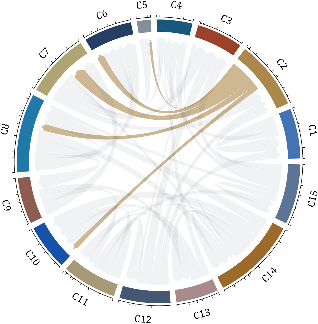
demo 15
CList = [0.81,0.72,0.83
0.69,0.82,0.89
0.17,0.44,0.64
0.70,0.85,0.55
0.03,0.57,0.13
0.97,0.67,0.64
0.84,0.09,0.12
1.00,0.80,0.46
0.98,0.52,0.01
];
figure('Units','normalized', 'Position',[.02,.05,.53,.85], 'Color',[1,1,1])
% =========================================================================
ax1 = axes('Parent',gcf, 'Position',[0,1/2,1/2,1/2]);
dataMat = rand([9,9]);
dataMat(dataMat > .4) = 0;
BCC = biChordChart(dataMat, 'Arrow','on', 'CData',CList);
BCC = BCC.draw();
BCC.tickState('on')
BCC.setFont('Visible','off')
% 修改弦颜色(Modify chord color)
for i = 1:size(dataMat, 1)
for j = 1:size(dataMat, 2)
if dataMat(i,j) > 0
BCC.setChordMN(i,j, 'FaceAlpha',.6)
end
end
end
text(-1.2,1.2, 'a', 'FontName','Times New Roman', 'FontSize',35)
% =========================================================================
ax2 = axes('Parent',gcf, 'Position',[1/2,1/2,1/2,1/2]);
dataMat = rand([9,9]);
dataMat(dataMat > .4) = 0;
dataMat = dataMat.*(1:9);
BCC = biChordChart(dataMat, 'Arrow','on', 'CData',CList);
BCC = BCC.draw();
BCC.tickState('on')
BCC.setFont('Visible','off')
% 修改弦颜色(Modify chord color)
for i = 1:size(dataMat, 1)
for j = 1:size(dataMat, 2)
if dataMat(i,j) > 0
BCC.setChordMN(i,j, 'FaceAlpha',.6)
end
end
end
text(-1.2,1.2, 'b', 'FontName','Times New Roman', 'FontSize',35)
% =========================================================================
ax3 = axes('Parent',gcf, 'Position',[0,0,1/2,1/2]);
dataMat = rand([9,9]);
dataMat(dataMat > .4) = 0;
dataMat = dataMat.*(1:9).';
BCC = biChordChart(dataMat, 'Arrow','on', 'CData',CList);
BCC = BCC.draw();
BCC.tickState('on')
BCC.setFont('Visible','off')
% 修改弦颜色(Modify chord color)
for i = 1:size(dataMat, 1)
for j = 1:size(dataMat, 2)
if dataMat(i,j) > 0
BCC.setChordMN(i,j, 'FaceAlpha',.6)
end
end
end
text(-1.2,1.2, 'c', 'FontName','Times New Roman', 'FontSize',35)
% =========================================================================
ax4 = axes('Parent',gcf, 'Position',[1/2,0,1/2,1/2]);
ax4.XColor = 'none'; ax4.YColor = 'none';
ax4.XLim = [-1,1]; ax4.YLim = [-1,1];
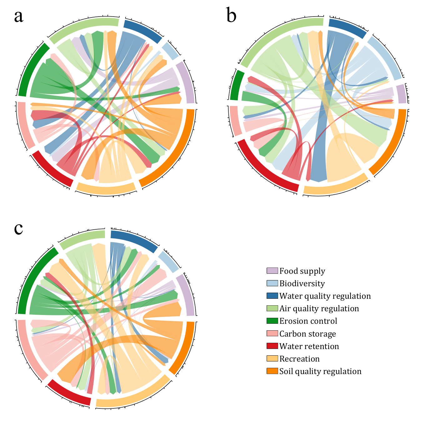
hold on
NameList = {'Food supply', 'Biodiversity', 'Water quality regulation', ...
'Air quality regulation', 'Erosion control', 'Carbon storage', ...
'Water retention', 'Recreation', 'Soil quality regulation'};
patchHdl = [];
for i = 1:size(dataMat, 2)
patchHdl(i) = fill([10,11,12],[10,13,13], CList(i,:), 'EdgeColor',[0,0,0]);
end
lgdHdl = legend(patchHdl, NameList, 'Location','best', 'FontSize',14, 'FontName','Cambria', 'Box','off');
lgdHdl.Position = [.625,.11,.255,.27];
lgdHdl.ItemTokenSize = [18,8];
demo 16
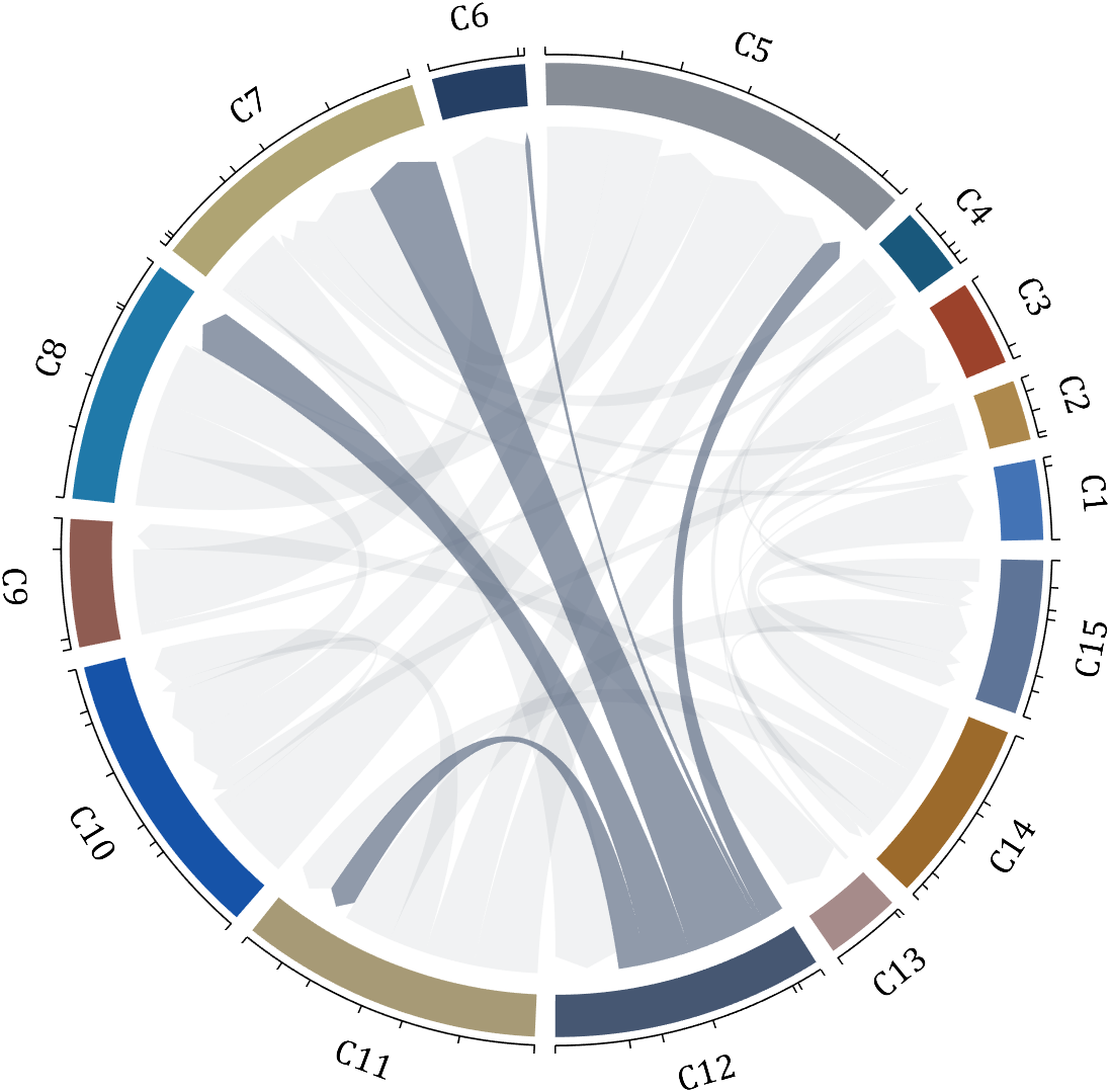
dataMat = rand([15,15]);
dataMat(dataMat > .2) = 0;
CList = [ 75,146,241; 252,180, 65; 224, 64, 10; 5,100,146; 191,191,191;
26, 59,105; 255,227,130; 18,156,221; 202,107, 75; 0, 92,219;
243,210,136; 80, 99,129; 241,185,168; 224,131, 10; 120,147,190]./255;
CListC = [54,69,92]./255;
CList = CList.*.6 + CListC.*.4;
figure('Units','normalized', 'Position',[.02,.05,.6,.85])
BCC = biChordChart(dataMat, 'Arrow','on', 'CData',CList);
BCC = BCC.draw();
% 添加刻度
BCC.tickState('on')
% 修改字体,字号及颜色
BCC.setFont('FontName','Cambria', 'FontSize',17, 'Color',[0,0,0])
% 修改弦颜色(Modify chord color)
for i = 1:size(dataMat, 1)
for j = 1:size(dataMat, 2)
if dataMat(i,j) > 0
BCC.setChordMN(i,j, 'FaceColor',CListC ,'FaceAlpha',.07)
end
end
end
[~, N] = max(sum(dataMat > 0, 2));
for j = 1:size(dataMat, 2)
BCC.setChordMN(N,j, 'FaceColor',CList(N,:) ,'FaceAlpha',.6)
end
You need to download following tools:
- - Chord chart: [chord chart](https://www.mathworks.com/matlabcentral/fileexchange/116550-chord-chart)
- - Directed graph chord chart: [digraph chord chart]:(https://www.mathworks.com/matlabcentral/fileexchange/121043-digraph-chord-chart)
MatGPT was launched on March 22, 2023 and I am amazed at how many times it has been downloaded since then - close to 16,000 downloads in one year. When AI Chat Playground came out on MATLAB Central, I thought surely that people will stop using MatGPT. Boy I was wrong.
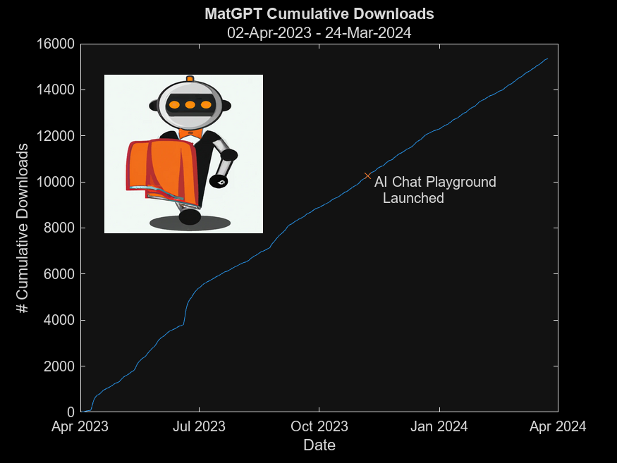
In early 2023 I was playing with the new shiny toy called ChatGPT like everyone else but instead of having it tell me jokes or haiku, I wanted to know how I can use it on MATLAB, and I started collecting the prompts that worked. Someone suggested I should turn that into an app, and MatGPT was born with help from other colleagues.
Here is the question - what should I do with it now? Some people suggested I could add other LLMs like Gemini or Claude, but I am more interested in learning how people actually use it.
If you are a MatGPT user, do you mind sharing how you use the app?
In short: support varying color in at least the plot, plot3, fplot, and fplot3 functions.
This has been a thing that's come up quite a few times, and includes questions/requests by users, workarounds by the community, and workarounds presented by MathWorks -- examples of each below. It's a feature that exists in Python's Matplotlib library and Sympy. Anyways, given that there are myriads of workarounds, it appears to be one of the most common requests for Matlab plots (Matlab's plotting is, IMO, one of the best features of the product), the request precedes the 21st century, and competitive tools provide the functionality, it would seem to me that this might be the next great feature for Matlab plotting.
I'm curious to get the rest of the community's thoughts... what's everyone else think about this?
---
User questions/requests
- https://www.mathworks.com/matlabcentral/answers/480389-colored-line-plot-according-to-a-third-variable
- https://www.mathworks.com/matlabcentral/answers/2092641-how-to-solve-a-problem-with-the-generation-of-multiple-colored-segments-on-one-line-in-matlab-plot
- https://www.mathworks.com/matlabcentral/answers/5042-how-do-i-vary-color-along-a-2d-line
- https://www.mathworks.com/matlabcentral/answers/1917650-how-to-plot-a-trajectory-with-varying-colour
- https://www.mathworks.com/matlabcentral/answers/1917650-how-to-plot-a-trajectory-with-varying-colour
- https://www.mathworks.com/matlabcentral/answers/511523-how-to-create-plot3-varying-color-figure
- https://www.mathworks.com/matlabcentral/answers/393810-multiple-colours-in-a-trajectory-plot
- https://www.mathworks.com/matlabcentral/answers/523135-creating-a-rainbow-colour-plot-trajectory
- https://www.mathworks.com/matlabcentral/answers/469929-how-to-vary-the-color-of-a-dynamic-line
- https://www.mathworks.com/matlabcentral/answers/585011-how-could-i-adjust-the-color-of-multiple-lines-within-a-graph-without-using-the-default-matlab-colo
- https://www.mathworks.com/matlabcentral/answers/517177-how-to-interpolate-color-along-a-curve-with-specific-colors
- https://www.mathworks.com/matlabcentral/answers/281645-variate-color-depending-on-the-y-value-in-plot
- https://www.mathworks.com/matlabcentral/answers/439176-how-do-i-vary-the-color-along-a-line-in-polar-coordinates
- https://www.mathworks.com/matlabcentral/answers/1849193-creating-rainbow-coloured-plots-in-3d
- https://groups.google.com/g/comp.soft-sys.matlab/c/cLgjSeEC15I?hl=en&pli=1 (a question asked in 1999!)
- ... the list goes on, and on, and on...
User-provided workarounds
- https://undocumentedmatlab.com/articles/plot-line-transparency-and-color-gradient
- https://www.mathworks.com/matlabcentral/fileexchange/19476-colored-line-or-scatter-plot
- https://www.mathworks.com/matlabcentral/fileexchange/23566-3d-colored-line-plot
- https://www.mathworks.com/matlabcentral/fileexchange/30423-conditionally-colored-line-plot
- https://www.mathworks.com/matlabcentral/fileexchange/14677-cline
- https://www.mathworks.com/matlabcentral/fileexchange/8597-plot-3d-color-line
- https://www.mathworks.com/matlabcentral/fileexchange/39972-colormapline-color-changing-2d-or-3d-line
- https://www.mathworks.com/matlabcentral/fileexchange/37725-conditionally-colored-plot-ccplot
- https://www.mathworks.com/matlabcentral/fileexchange/11611-linear-2d-plot-with-rainbow-color
- https://www.mathworks.com/matlabcentral/fileexchange/26692-color_line
- https://www.mathworks.com/matlabcentral/fileexchange/32911-plot3rgb
- And perhaps more?
MathWorks-provided workarounds
- https://www.mathworks.com/videos/coloring-a-line-based-on-height-gradient-or-some-other-value-in-matlab-97128.html
- https://www.mathworks.com/videos/making-a-multi-color-line-in-matlab-97127.html
- https://www.mathworks.com/matlabcentral/fileexchange/95663-color-trajectory-plot (contributed by a MathWorks staff member)
- And perhaps more?
I was in a meeting the other day and a coworker shared a smiley face they created using the AI Chat Playground. The image looked something like this:
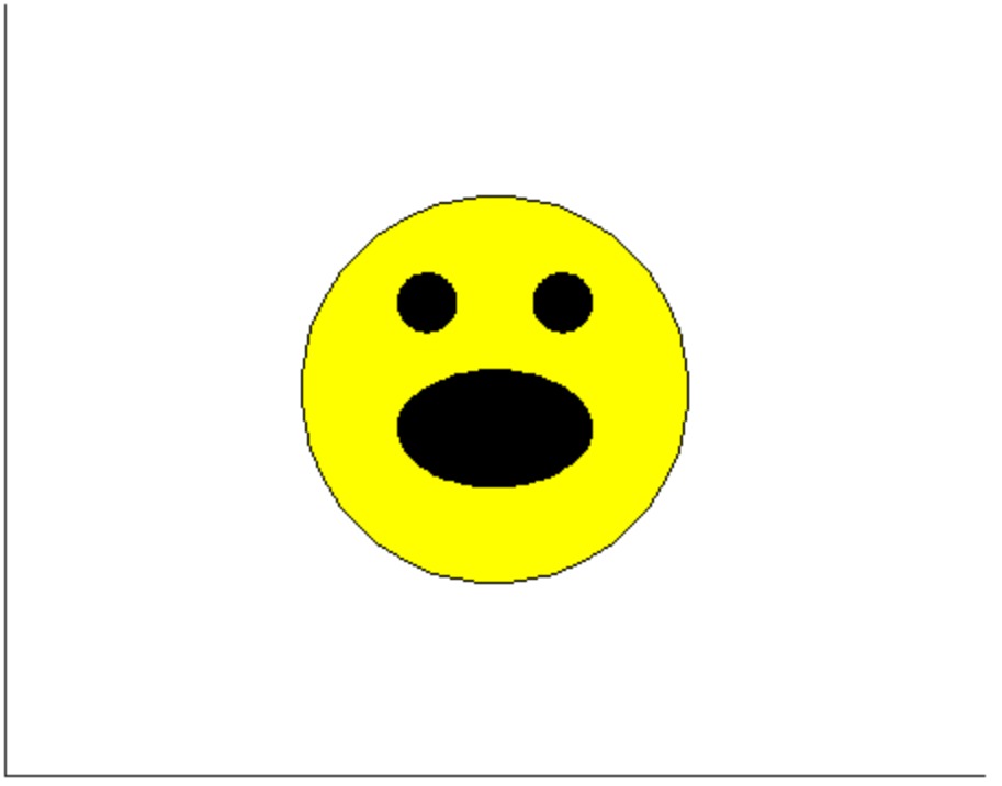
And I suspect the prompt they used was something like this:
"Create a smiley face"
I imagine this output wasn't what my coworker had expected so he was left thinking that this was as good as it gets without manually editing the code, and that the AI Chat Playground couldn't do any better.
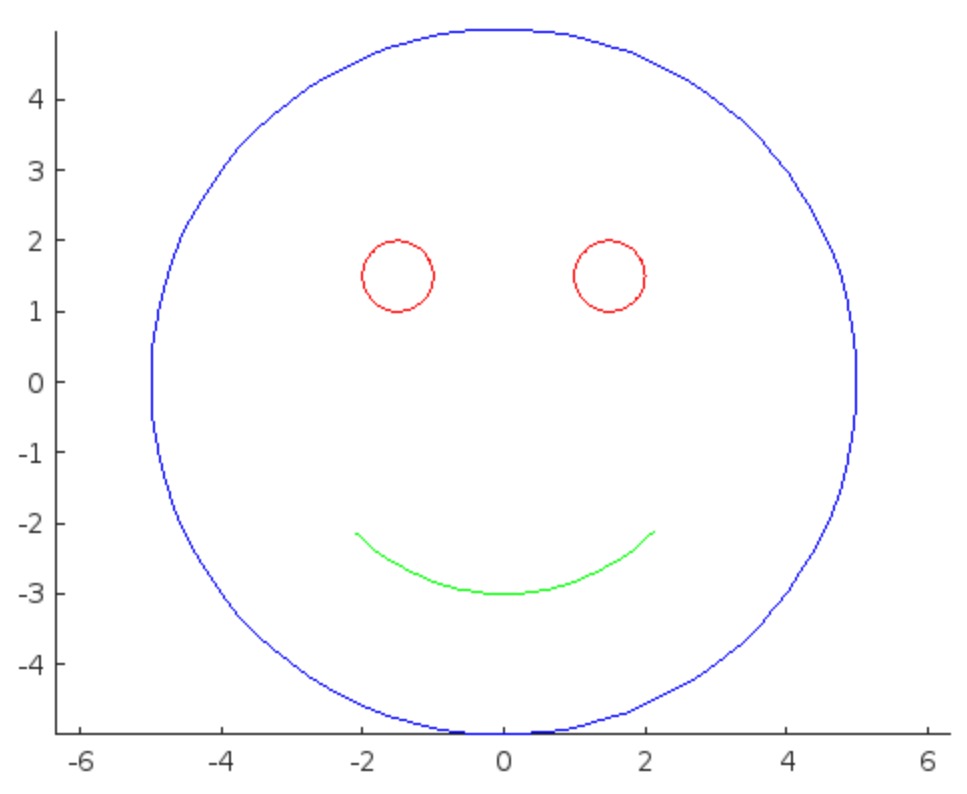
I thought I could get a better result using the Playground so I tried a more detailed prompt using a multi-step technique like this:
"Follow these instructions:
- Create code that plots a circle
- Create two smaller circles as eyes within the first circle
- Create an arc that looks like a smile in the lower part of the first circle"
The output of this prompt was better in my opinion.
These queries/prompts are examples of 'zero-shot' prompts, the expectation being a good result with just one query. As opposed to a back-and-forth chat session working towards a desired outcome.
I wonder how many attempts everyone tries before they decide they can't anything more from the AI/LLM. There are times I'll send dozens of chat queries if I feel like I'm getting close to my goal, while other times I'll try just one or two. One thing I always find useful is seeing how others interact with AI models, which is what inspired me to share this.
Does anyone have examples of techniques that work well? I find multi-step instructions often produces good results.
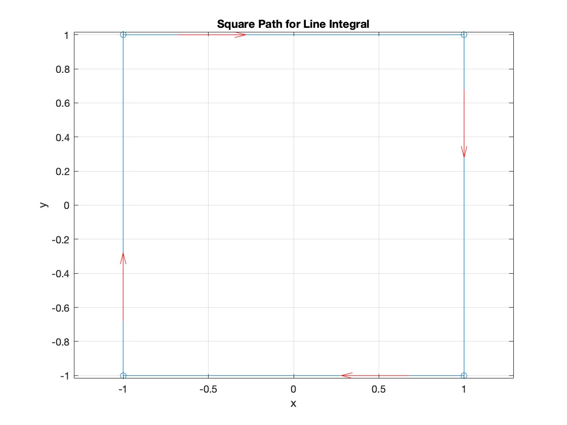
The line integral 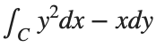 , where C is the boundary of the square
  oriented counterclockwise, can be evaluated in two ways:
, where C is the boundary of the square Using the definition of the line integral:
% Initialize the integral sum
integral_sum = 0;
% Segment C1: x = -1, y goes from -1 to 1
y = linspace(-1, 1);
x = -1 * ones(size(y));
dy = diff(y);
integral_sum = integral_sum + sum(-x(1:end-1) .* dy);
% Segment C2: y = 1, x goes from -1 to 1
x = linspace(-1, 1);
y = ones(size(x));
dx = diff(x);
integral_sum = integral_sum + sum(y(1:end-1).^2 .* dx);
% Segment C3: x = 1, y goes from 1 to -1
y = linspace(1, -1);
x = ones(size(y));
dy = diff(y);
integral_sum = integral_sum + sum(-x(1:end-1) .* dy);
% Segment C4: y = -1, x goes from 1 to -1
x = linspace(1, -1);
y = -1 * ones(size(x));
dx = diff(x);
integral_sum = integral_sum + sum(y(1:end-1).^2 .* dx);
disp(['Direct Method Integral: ', num2str(integral_sum)]);
Plotting the square path
% Define the square's vertices
vertices = [-1 -1; -1 1; 1 1; 1 -1; -1 -1];
% Plot the square
figure;
plot(vertices(:,1), vertices(:,2), '-o');
title('Square Path for Line Integral');
xlabel('x');
ylabel('y');
grid on;
axis equal;
% Add arrows to indicate the path direction (counterclockwise)
hold on;
for i = 1:size(vertices,1)-1
% Calculate direction
dx = vertices(i+1,1) - vertices(i,1);
dy = vertices(i+1,2) - vertices(i,2);
% Reduce the length of the arrow for better visibility
scale = 0.2;
dx = scale * dx;
dy = scale * dy;
% Calculate the start point of the arrow
startx = vertices(i,1) + (1 - scale) * dx;
starty = vertices(i,2) + (1 - scale) * dy;
% Plot the arrow
quiver(startx, starty, dx, dy, 'MaxHeadSize', 0.5, 'Color', 'r', 'AutoScale', 'off');
end
hold off;
Apply Green's Theorem for the line integral
% Define the partial derivatives of P and Q
f = @(x, y) -1 - 2*y; % derivative of -x with respect to x is -1, and derivative of y^2 with respect to y is 2y
% Compute the double integral over the square [-1,1]x[-1,1]
integral_value = integral2(f, -1, 1, 1, -1);
disp(['Green''s Theorem Integral: ', num2str(integral_value)]);
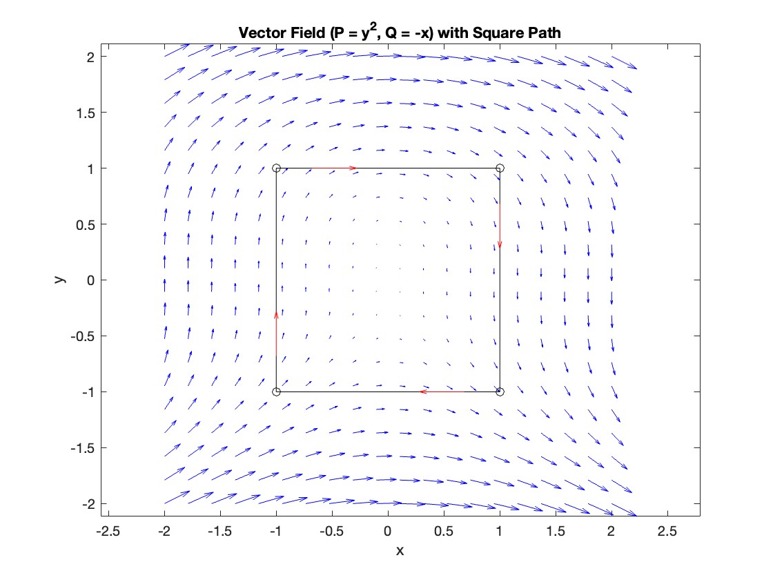
Plotting the vector field related to Green’s theorem
% Define the grid for the vector field
[x, y] = meshgrid(linspace(-2, 2, 20), linspace(-2 ,2, 20));
% Define the vector field components
P = y.^2; % y^2 component
Q = -x; % -x component
% Plot the vector field
figure;
quiver(x, y, P, Q, 'b');
hold on; % Hold on to plot the square on the same figure
% Define the square's vertices
vertices = [-1 -1; -1 1; 1 1; 1 -1; -1 -1];
% Plot the square path
plot(vertices(:,1), vertices(:,2), '-o', 'Color', 'k'); % 'k' for black color
title('Vector Field (P = y^2, Q = -x) with Square Path');
xlabel('x');
ylabel('y');
axis equal;
% Add arrows to indicate the path direction (counterclockwise)
for i = 1:size(vertices,1)-1
% Calculate direction
dx = vertices(i+1,1) - vertices(i,1);
dy = vertices(i+1,2) - vertices(i,2);
% Reduce the length of the arrow for better visibility
scale = 0.2;
dx = scale * dx;
dy = scale * dy;
% Calculate the start point of the arrow
startx = vertices(i,1) + (1 - scale) * dx;
starty = vertices(i,2) + (1 - scale) * dy;
% Plot the arrow
quiver(startx, starty, dx, dy, 'MaxHeadSize', 0.5, 'Color', 'r', 'AutoScale', 'off');
end
hold off;
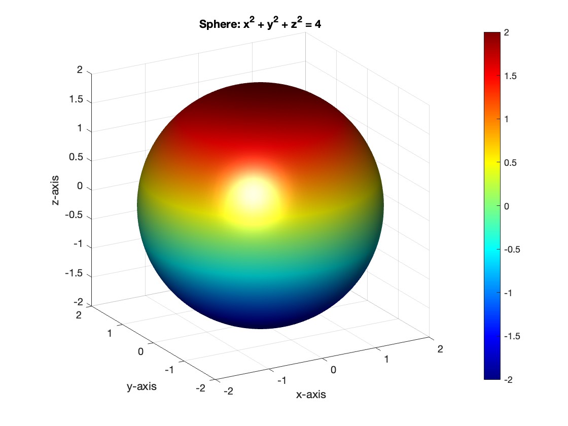
To solve a surface integral for example the over the sphere
  easily in MATLAB, you can leverage the symbolic toolbox for a direct and clear solution. Here is a tip to simplify the process:
over the sphere - Use Symbolic Variables and Functions: Define your variables symbolically, including the parameters of your spherical coordinates θ and ϕ and the radius r . This allows MATLAB to handle the expressions symbolically, making it easier to manipulate and integrate them.
- Express in Spherical Coordinates Directly: Since you already know the sphere's equation and the relationship in spherical coordinates, define x, y, and z in terms of r , θ and ϕ directly.
- Perform Symbolic Integration: Use MATLAB's `int` function to integrate symbolically. Since the sphere and the function
 are symmetric, you can exploit these symmetries to simplify the calculation.
Here’s how you can apply this tip in MATLAB code:
% Include the symbolic math toolbox
syms theta phi
% Define the limits for theta and phi
theta_limits = [0, pi];
phi_limits = [0, 2*pi];
% Define the integrand function symbolically
integrand = 16 * sin(theta)^3 * cos(phi)^2;
% Perform the symbolic integral for the surface integral
surface_integral = int(int(integrand, theta, theta_limits(1), theta_limits(2)), phi, phi_limits(1), phi_limits(2));
% Display the result of the surface integral symbolically
disp(['The surface integral of x^2 over the sphere is ', char(surface_integral)]);
% Number of points for plotting
num_points = 100;
% Define theta and phi for the sphere's surface
[theta_mesh, phi_mesh] = meshgrid(linspace(double(theta_limits(1)), double(theta_limits(2)), num_points), ...
linspace(double(phi_limits(1)), double(phi_limits(2)), num_points));
% Spherical to Cartesian conversion for plotting
r = 2; % radius of the sphere
x = r * sin(theta_mesh) .* cos(phi_mesh);
y = r * sin(theta_mesh) .* sin(phi_mesh);
z = r * cos(theta_mesh);
% Plot the sphere
figure;
surf(x, y, z, 'FaceColor', 'interp', 'EdgeColor', 'none');
colormap('jet'); % Color scheme
shading interp; % Smooth shading
camlight headlight; % Add headlight-type lighting
lighting gouraud; % Use Gouraud shading for smooth color transitions
title('Sphere: x^2 + y^2 + z^2 = 4');
xlabel('x-axis');
ylabel('y-axis');
zlabel('z-axis');
colorbar; % Add color bar to indicate height values
axis square; % Maintain aspect ratio to be square
view([-30, 20]); % Set a nice viewing angle
I am often talking to new MATLAB users. I have put together one script. If you know how this script works, why, and what each line means, you will be well on your way on your MATLAB learning journey.
% Clear existing variables and close figures
clear;
close all;
% Print to the Command Window
disp('Hello, welcome to MATLAB!');
% Create a simple vector and matrix
vector = [1, 2, 3, 4, 5];
matrix = [1, 2, 3; 4, 5, 6; 7, 8, 9];
% Display the created vector and matrix
disp('Created vector:');
disp(vector);
disp('Created matrix:');
disp(matrix);
% Perform element-wise multiplication
result = vector .* 2;
% Display the result of the operation
disp('Result of element-wise multiplication of the vector by 2:');
disp(result);
% Create plot
x = 0:0.1:2*pi; % Generate values from 0 to 2*pi
y = sin(x); % Calculate the sine of these values
% Plotting
figure; % Create a new figure window
plot(x, y); % Plot x vs. y
title('Simple Plot of sin(x)'); % Give the plot a title
xlabel('x'); % Label the x-axis
ylabel('sin(x)'); % Label the y-axis
grid on; % Turn on the grid
disp('This is the end of the script. Explore MATLAB further to learn more!');
I would like to propose the creation of MATLAB EduHub, a dedicated channel within the MathWorks community where educators, students, and professionals can share and access a wealth of educational material that utilizes MATLAB. This platform would act as a central repository for articles, teaching notes, and interactive learning modules that integrate MATLAB into the teaching and learning of various scientific fields.
Key Features:
1. Resource Sharing: Users will be able to upload and share their own educational materials, such as articles, tutorials, code snippets, and datasets.
2. Categorization and Search: Materials can be categorized for easy searching by subject area, difficulty level, and MATLAB version..
3. Community Engagement: Features for comments, ratings, and discussions to encourage community interaction.
4. Support for Educators: Special sections for educators to share teaching materials and track engagement.
Benefits:
- Enhanced Educational Experience: The platform will enrich the learning experience through access to quality materials.
- Collaboration and Networking: It will promote collaboration and networking within the MATLAB community.
- Accessibility of Resources: It will make educational materials available to a wider audience.
By establishing MATLAB EduHub, I propose a space where knowledge and experience can be freely shared, enhancing the educational process and the MATLAB community as a whole.
Happy Pi Day!
3.14 π Day has arrived, and this post provides some very cool pi implementations and complete MATLAB code.
Firstly, in order to obtain the first n decimal places of pi, we need to write the following code (to prevent inaccuracies, we need to take a few more tails and perform another operation of taking the first n decimal places when needed):
function Pi=getPi(n)
if nargin<1,n=3;end
Pi=char(vpa(sym(pi),n+10));
Pi=abs(Pi)-48;
Pi=Pi(3:n+2);
end
With this function to obtain the decimal places of pi, our visualization journey has begun~Step by step, from simple to complex~(Please try to use newer versions of MATLAB to run, at least R17b)
1 Pie chart
Just calculate the proportion of each digit to the first 1500 decimal places:
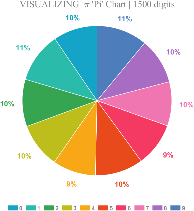
% 获取pi前1500位小数
Pi=getPi(1500);
% 统计各个数字出现次数
numNum=find([diff(sort(Pi)),1]);
numNum=[numNum(1),diff(numNum)];
% 配色列表
CM=[20,164,199;43,187,170;53,165,81;189,190,28;248,167,22;
232,74,27;244,57,99;240,118,177;168,109,195;78,125,187]./255;
% 绘图并修饰
pieHdl=pie(numNum);
set(gcf,'Color',[1,1,1],'Position',[200,100,620,620]);
for i=1:2:20
pieHdl(i).EdgeColor=[1,1,1];
pieHdl(i).LineWidth=1;
pieHdl(i).FaceColor=CM((i+1)/2,:);
end
for i=2:2:20
pieHdl(i).Color=CM(i/2,:);
pieHdl(i).FontWeight='bold';
pieHdl(i).FontSize=14;
end
% 绘制图例并修饰
lgdHdl=legend(num2cell('0123456789'));
lgdHdl.FontWeight='bold';
lgdHdl.FontSize=11;
lgdHdl.TextColor=[.5,.5,.5];
lgdHdl.Location='southoutside';
lgdHdl.Box='off';
lgdHdl.NumColumns=10;
lgdHdl.ItemTokenSize=[20,15];
title("VISUALIZING \pi 'Pi' Chart | 1500 digits",'FontSize',18,...
'FontName','Times New Roman','Color',[.5,.5,.5])
2 line chart
Calculate the change in the proportion of each number:
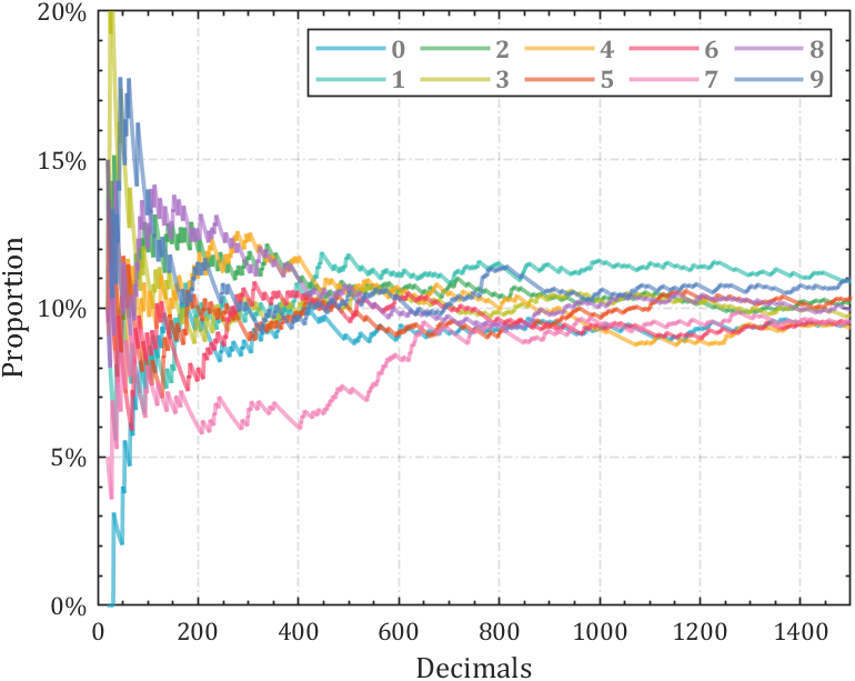
% 获取pi前1500位小数
Pi=getPi(1500);
% 计算比例变化
Ratio=cumsum(Pi==(0:9)',2);
Ratio=Ratio./sum(Ratio);
D=1:length(Ratio);
% 配色列表
CM=[20,164,199;43,187,170;53,165,81;189,190,28;248,167,22;
232,74,27;244,57,99;240,118,177;168,109,195;78,125,187]./255;
hold on
% 循环绘图
for i=1:10
plot(D(20:end),Ratio(i,20:end),'Color',[CM(i,:),.6],'LineWidth',1.8)
end
% 坐标区域修饰
ax=gca;box on;grid on
ax.YLim=[0,.2];
ax.YTick=0:.05:.2;
ax.XTick=0:200:1400;
ax.YTickLabel={'0%','5%','10%','15%','20%'};
ax.XMinorTick='on';
ax.YMinorTick='on';
ax.LineWidth=.8;
ax.GridLineStyle='-.';
ax.FontName='Cambria';
ax.FontSize=11;
ax.XLabel.String='Decimals';
ax.YLabel.String='Proportion';
ax.XLabel.FontSize=13;
ax.YLabel.FontSize=13;
% 绘制图例并修饰
lgdHdl=legend(num2cell('0123456789'));
lgdHdl.NumColumns=5;
lgdHdl.FontWeight='bold';
lgdHdl.FontSize=11;
lgdHdl.TextColor=[.5,.5,.5];
3 stacked area diagram
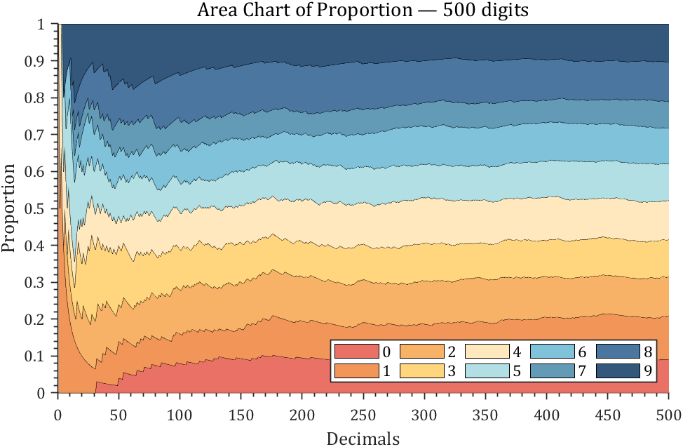
% 获取pi前500位小数
Pi=getPi(500);
% 计算比例变化
Ratio=cumsum(Pi==(0:9)',2);
Ratio=Ratio./sum(Ratio);
% 配色列表
CM=[231,98,84;239,138,71;247,170,88;255,208,111;255,230,183;
170,220,224;114,188,213;82,143,173;55,103,149;30,70,110]./255;
% 绘制堆叠面积图
hold on
areaHdl=area(Ratio');
for i=1:10
areaHdl(i).FaceColor=CM(i,:);
areaHdl(i).FaceAlpha=.9;
end
% 图窗和坐标区域修饰
set(gcf,'Position',[200,100,720,420]);
ax=gca;
ax.YLim=[0,1];
ax.XMinorTick='on';
ax.YMinorTick='on';
ax.LineWidth=.8;
ax.FontName='Cambria';
ax.FontSize=11;
ax.TickDir='out';
ax.XLabel.String='Decimals';
ax.YLabel.String='Proportion';
ax.XLabel.FontSize=13;
ax.YLabel.FontSize=13;
ax.Title.String='Area Chart of Proportion — 500 digits';
ax.Title.FontSize=14;
% 绘制图例并修饰
lgdHdl=legend(num2cell('0123456789'));
lgdHdl.NumColumns=5;
lgdHdl.FontSize=11;
lgdHdl.Location='southeast';
4 connected stacked bar chart
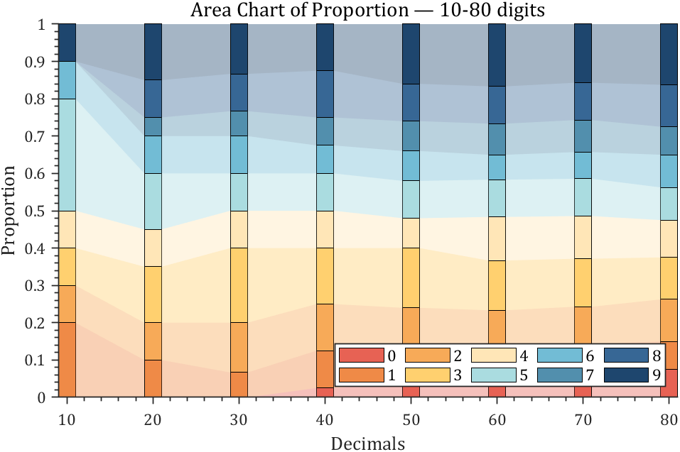
% 获取pi前100位小数
Pi=getPi(100);
% 计算比例变化
Ratio=cumsum(Pi==(0:9)',2);
Ratio=Ratio./sum(Ratio);
X=Ratio(:,10:10:80)';
barHdl=bar(X,'stacked','BarWidth',.2);
CM=[231,98,84;239,138,71;247,170,88;255,208,111;255,230,183;
170,220,224;114,188,213;82,143,173;55,103,149;30,70,110]./255;
for i=1:10
barHdl(i).FaceColor=CM(i,:);
end
% 以下是生成连接的部分
hold on;axis tight
yEndPoints=reshape([barHdl.YEndPoints]',length(barHdl(1).YData),[])';
zeros(1,length(barHdl(1).YData));
yEndPoints=[zeros(1,length(barHdl(1).YData));yEndPoints];
barWidth=barHdl(1).BarWidth;
for i=1:length(barHdl)
for j=1:length(barHdl(1).YData)-1
y1=min(yEndPoints(i,j),yEndPoints(i+1,j));
y2=max(yEndPoints(i,j),yEndPoints(i+1,j));
if y1*y2<0
ty=yEndPoints(find(yEndPoints(i+1,j)*yEndPoints(1:i,j)>=0,1,'last'),j);
y1=min(ty,yEndPoints(i+1,j));
y2=max(ty,yEndPoints(i+1,j));
end
y3=min(yEndPoints(i,j+1),yEndPoints(i+1,j+1));
y4=max(yEndPoints(i,j+1),yEndPoints(i+1,j+1));
if y3*y4<0
ty=yEndPoints(find(yEndPoints(i+1,j+1)*yEndPoints(1:i,j+1)>=0,1,'last'),j+1);
y3=min(ty,yEndPoints(i+1,j+1));
y4=max(ty,yEndPoints(i+1,j+1));
end
fill([j+.5.*barWidth,j+1-.5.*barWidth,j+1-.5.*barWidth,j+.5.*barWidth],...
[y1,y3,y4,y2],barHdl(i).FaceColor,'FaceAlpha',.4,'EdgeColor','none');
end
end
% 图窗和坐标区域修饰
set(gcf,'Position',[200,100,720,420]);
ax=gca;box off
ax.YLim=[0,1];
ax.XMinorTick='on';
ax.YMinorTick='on';
ax.LineWidth=.8;
ax.FontName='Cambria';
ax.FontSize=11;
ax.TickDir='out';
ax.XTickLabel={'10','20','30','40','50','60','70','80'};
ax.XLabel.String='Decimals';
ax.YLabel.String='Proportion';
ax.XLabel.FontSize=13;
ax.YLabel.FontSize=13;
ax.Title.String='Area Chart of Proportion — 10-80 digits';
ax.Title.FontSize=14;
% 绘制图例并修饰
lgdHdl=legend(barHdl,num2cell('0123456789'));
lgdHdl.NumColumns=5;
lgdHdl.FontSize=11;
lgdHdl.Location='southeast';
5 bichord chart
Need to use this tool:
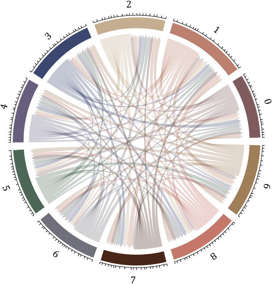
% 构建连接矩阵
dataMat=zeros(10,10);
Pi=getPi(1001);
for i=1:1000
dataMat(Pi(i)+1,Pi(i+1)+1)=dataMat(Pi(i)+1,Pi(i+1)+1)+1;
end
BCC=biChordChart(dataMat,'Arrow','on','Label',num2cell('0123456789'));
BCC=BCC.draw();
% 添加刻度
BCC.tickState('on')
% 修改字体,字号及颜色
BCC.setFont('FontName','Cambria','FontSize',17)
set(gcf,'Position',[200,100,820,820]);
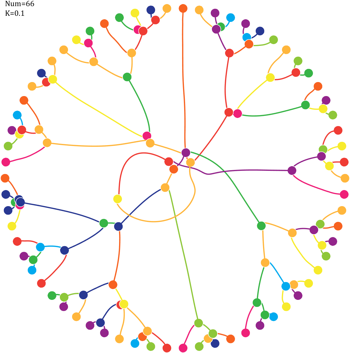
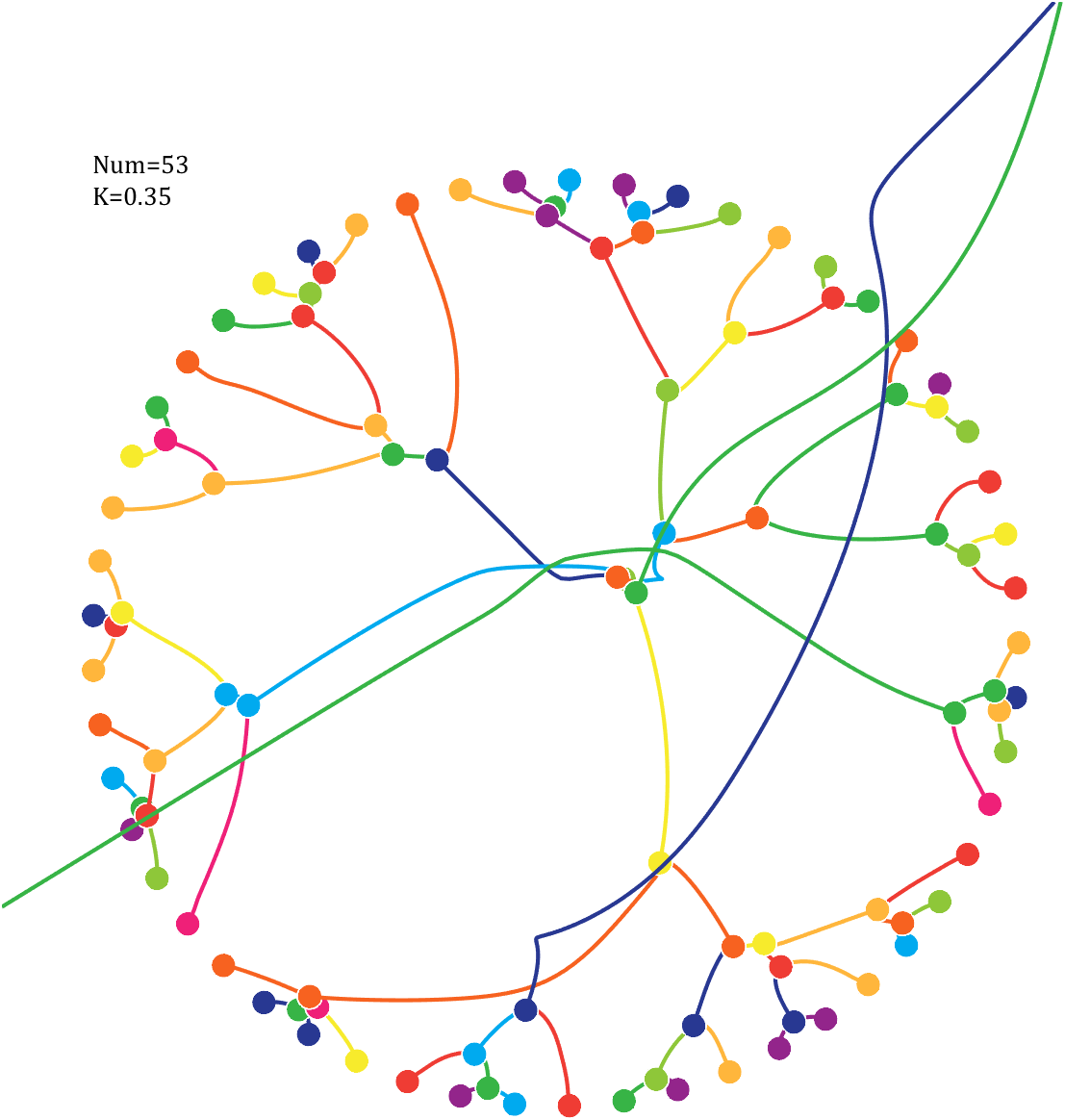
6 Gravity simulation diagram
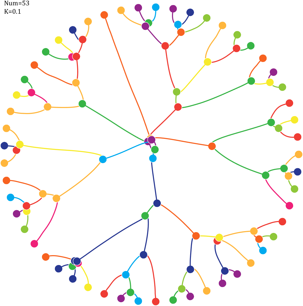
Imagine each decimal as a small ball with a mass of
For example, if , the weight of ball 0 is 1, ball 9 is 1.2589, the initial velocity of the ball is 0, and it is attracted by other balls. Gravity follows the inverse square law, and if the balls are close enough, they will collide and their value will become
After adding, take the mod, add the velocity direction proportionally, and recalculate the weight.
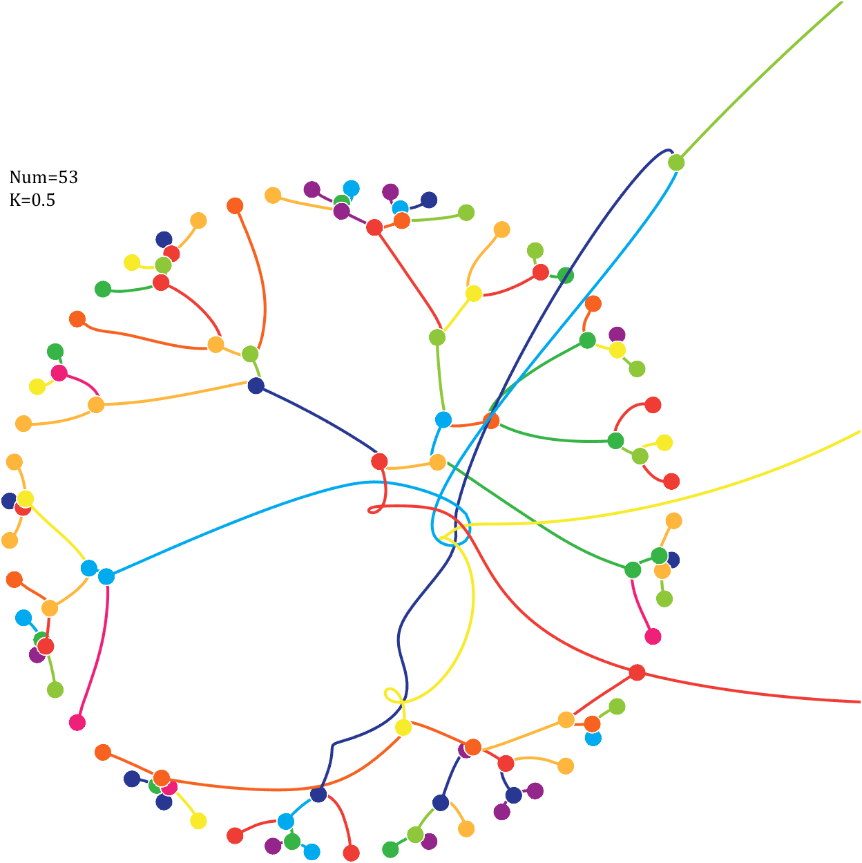
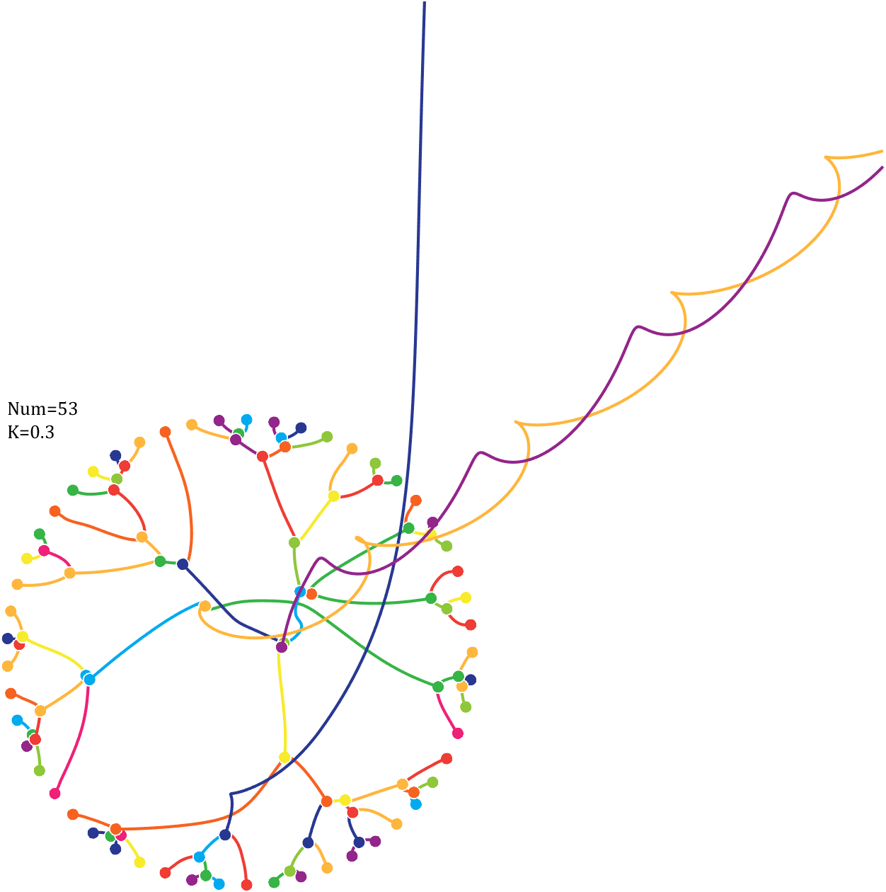
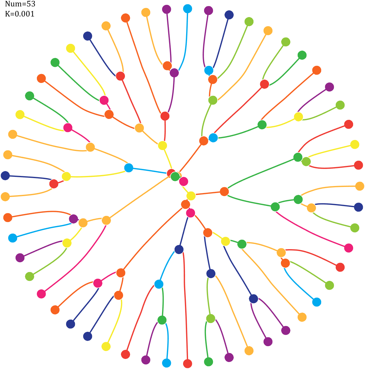
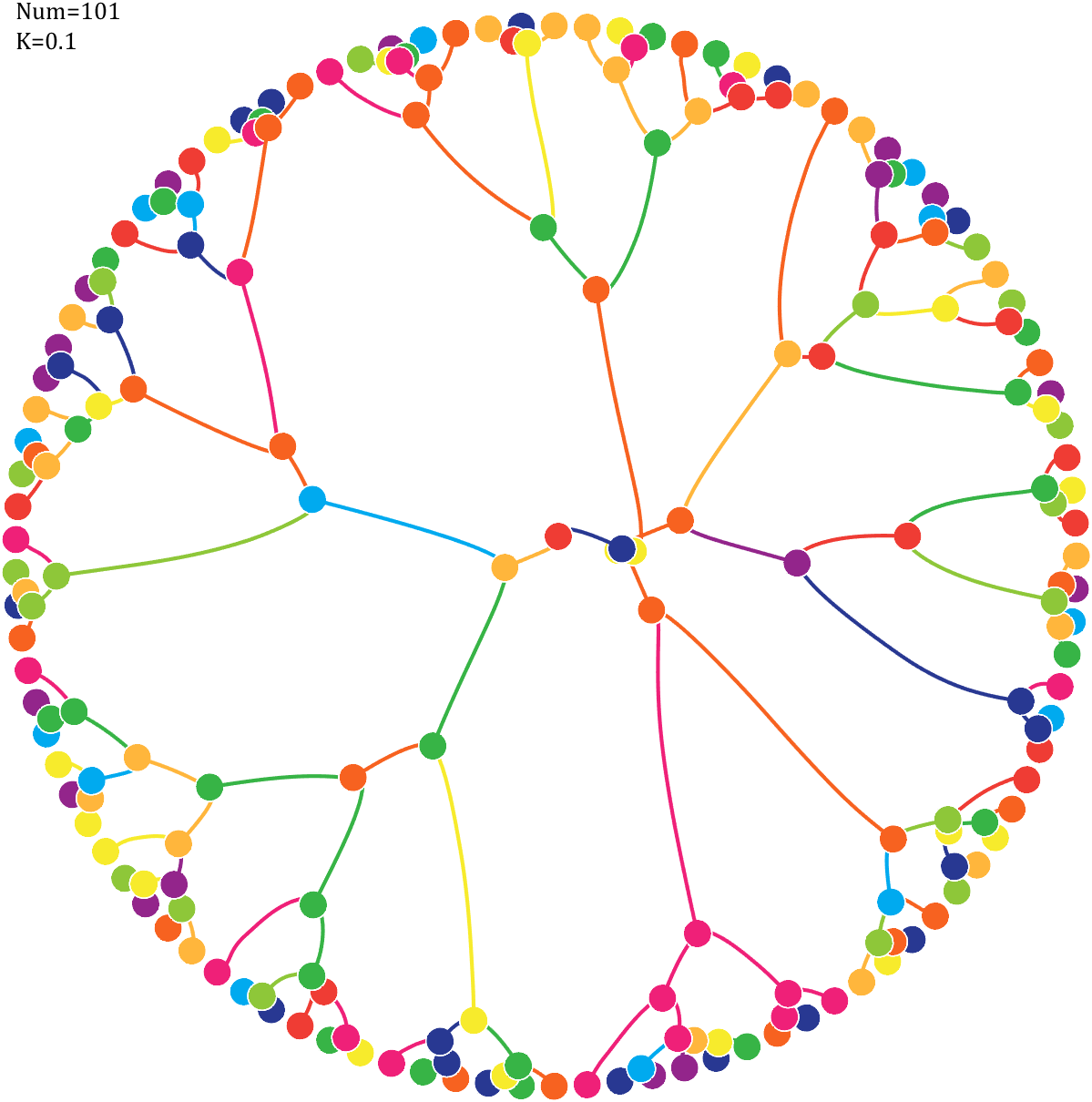
Pi=[3,getPi(71)];K=.18;
% 基础配置
CM=[239,32,120;239,60,52;247,98,32;255,182,60;247,235,44;
142,199,57;55,180,70;0,170,239;40,56,146;147,37,139]./255;
T=linspace(0,2*pi,length(Pi)+1)';
T=T(1:end-1);
ct=linspace(0,2*pi,100);
cx=cos(ct).*.027;
cy=sin(ct).*.027;
% 初始数据
Pi=Pi(:);
N=Pi;
X=cos(T);Y=sin(T);
VX=T.*0;VY=T.*0;
PX=X;PY=Y;
% 未碰撞时初始质量
getM=@(x)(x+1).^K;
M=getM(N);
% 绘制初始圆圈
hold on
for i=1:length(N)
fill(cx+X(i),cy+Y(i),CM(N(i)+1,:),'EdgeColor','w','LineWidth',1)
end
for k=1:800
% 计算加速度
Rn2=1./squareform(pdist([X,Y])).^2;
Rn2(eye(length(X))==1)=0;
MRn2=Rn2.*(M');
AX=X'-X;AY=Y'-Y;
normXY=sqrt(AX.^2+AY.^2);
AX=AX./normXY;AX(eye(length(X))==1)=0;
AY=AY./normXY;AY(eye(length(X))==1)=0;
AX=sum(AX.*MRn2,2)./150000;
AY=sum(AY.*MRn2,2)./150000;
% 计算速度及新位置
VX=VX+AX;X=X+VX;PX=[PX,X];
VY=VY+AY;Y=Y+VY;PY=[PY,Y];
% 检测是否有碰撞
R=squareform(pdist([X,Y]));
R(triu(ones(length(X)))==1)=inf;
[row,col]=find(R<=0.04);
if length(X)==1
break;
end
if ~isempty(row)
% 碰撞的点合为一体
XC=(X(row)+X(col))./2;YC=(Y(row)+Y(col))./2;
VXC=(VX(row).*M(row)+VX(col).*M(col))./(M(row)+M(col));
VYC=(VY(row).*M(row)+VY(col).*M(col))./(M(row)+M(col));
PC=nan(length(row),size(PX,2));
NC=mod(N(row)+N(col),10);
% 删除碰撞点并绘图
uniNum=unique([row;col]);
X(uniNum)=[];VX(uniNum)=[];
Y(uniNum)=[];VY(uniNum)=[];
for i=1:length(uniNum)
plot(PX(uniNum(i),:),PY(uniNum(i),:),'LineWidth',2,'Color',CM(N(uniNum(i))+1,:))
end
PX(uniNum,:)=[];PY(uniNum,:)=[];N(uniNum,:)=[];
% 绘制圆形
for i=1:length(XC)
fill(cx+XC(i),cy+YC(i),CM(NC(i)+1,:),'EdgeColor','w','LineWidth',1)
end
% 补充合体点
X=[X;XC];Y=[Y;YC];VX=[VX;VXC];VY=[VY;VYC];
PX=[PX;PC];PY=[PY;PC];N=[N;NC];M=getM(N);
end
end
for i=1:size(PX,1)
plot(PX(i,:),PY(i,:),'LineWidth',2,'Color',CM(N(i)+1,:))
end
text(-1,1,{['Num=',num2str(length(Pi))];['K=',num2str(K)]},'FontSize',13,'FontName','Cambria')
% 图窗及坐标区域修饰
set(gcf,'Position',[200,100,820,820]);
ax=gca;
ax.Position=[0,0,1,1];
ax.DataAspectRatio=[1,1,1];
ax.XLim=[-1.1,1.1];
ax.YLim=[-1.1,1.1];
ax.XTick=[];
ax.YTick=[];
ax.XColor='none';
ax.YColor='none';
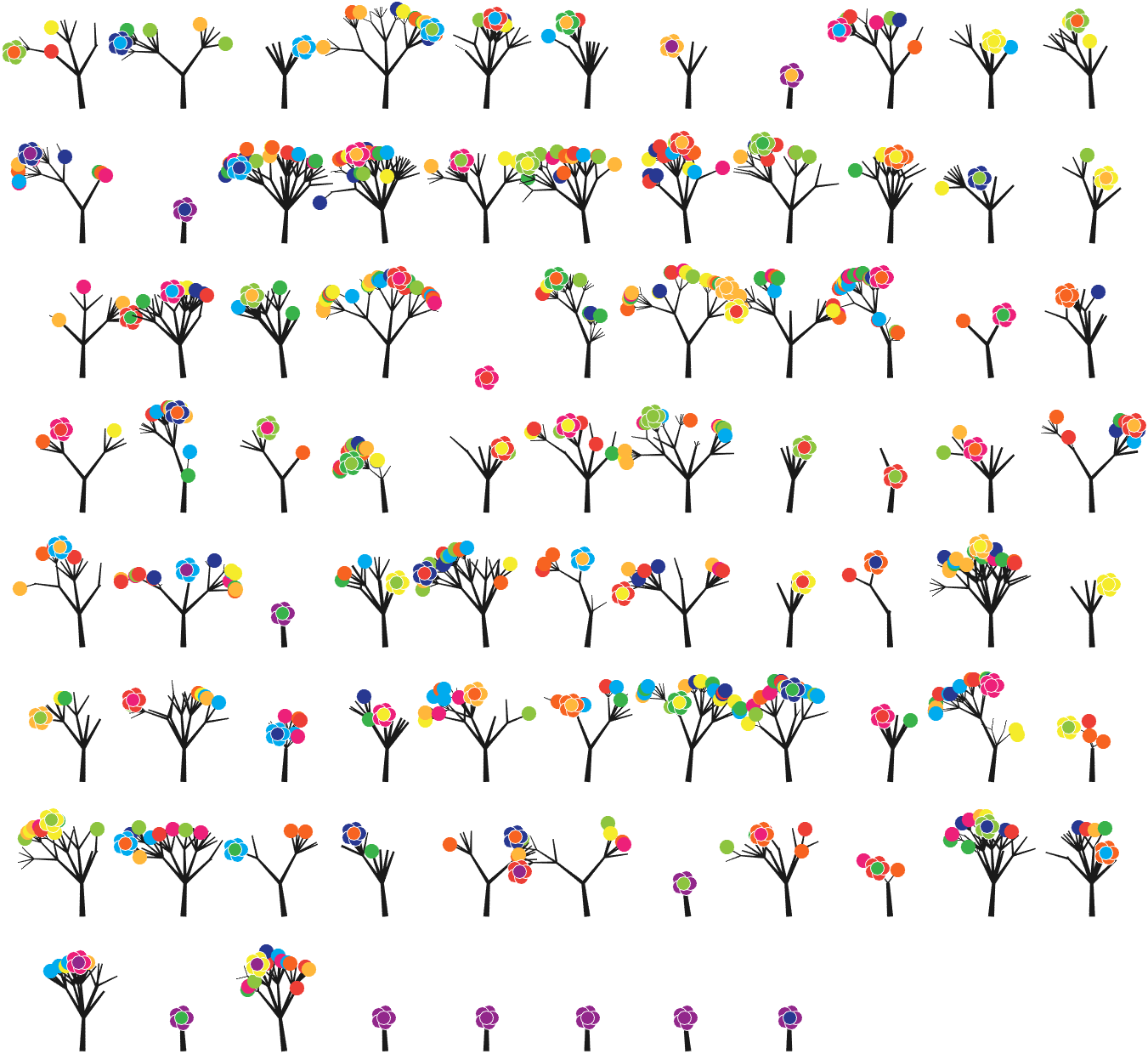
7 forest chart

The method comes from
The digits of π are shown as a forest. Each tree in the forest represents the digits of π up to the next 9. The first 10 trees are "grown" from the digit sets 314159, 2653589, 79, 3238462643383279, 50288419, 7169, 39, 9, 3751058209, and 749.
BRANCHES
The first digit of a tree controls how many branches grow from the trunk of the tree. For example, the first tree's first digit is 3, so you see 3 branches growing from the trunk.
The next digit's branches grow from the end of a branch of the previous digit in left-to-right order. This process continues until all the tree's digits have been used up.
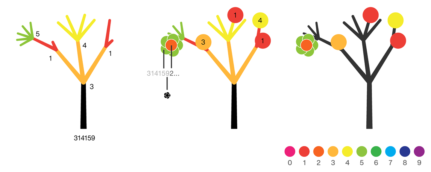
Each tree grows from a set of consecutive digits sampled from the digits of π up to the next 9. The first tree, shown here, grows from 314159. Each of the digits determine how many branches grow at each fork in the tree — the branches here are colored by their corresponding digit to illustrate this. Leaves encode the digits in a left-to-right order. The digit 9 spawns a flower on one of the branches of the previous digit. The branching exception is 0, which terminates the current branch — 0 branches grow!
LEAVES AND FLOWERS
The tree's digits themselves are drawn as circular leaves, color-coded by the digit.
The leaf exception is 9, which causes one of the branches of the previous digit to sprout a flower! The petals of the flower are colored by the digit before the 9 and the center is colored by the digit after the 9, which is on the next tree. This is how the forest propagates.
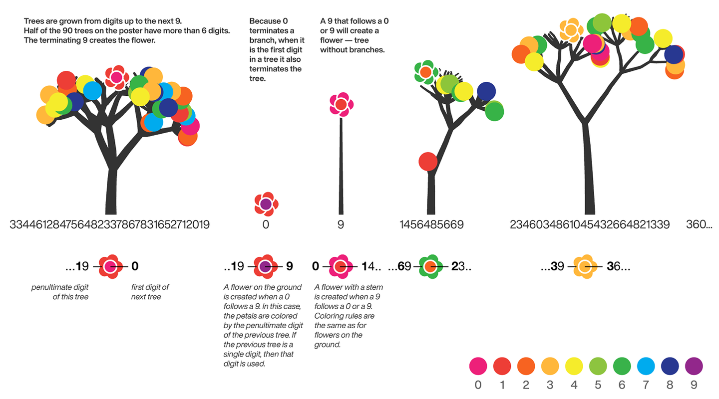
The colors of a flower are determined by the first digit of the next tree and the penultimate digit of the current tree. If the current tree only has one digit, then that digit is used. Leaves are placed at the tips of branches in a left-to-right order — you can "easily" read them off. Additionally, the leaves are distributed within the tree (without disturbing their left-to-right order) to spread them out as much as possible and avoid overlap. This order is deterministic.
The leaf placement exception are the branch set that sprouted the flower. These are not used to grow leaves — the flower needs space!
function PiTree(X,pos,D)
lw=2;
theta=pi/2+(rand(1)-.5).*pi./12;
% 树叶及花朵颜色
CM=[237,32,121;237,62,54;247,99,33;255,183,59;245,236,43;
141,196,63;57,178,74;0,171,238;40,56,145;146,39,139]./255;
hold on
if all(X(1:end-2)==0)
endSet=[pos,pos,theta];
else
kplot(pos(1)+[0,cos(theta)],pos(2)+[0,sin(theta)],lw./.6)
endSet=[pos,pos+[cos(theta),sin(theta)],theta];
% 计算层级
Layer=0;
for i=1:length(X)
Layer=[Layer,ones(1,X(i)).*i];
end
% 计算树枝
if D
for i=1:length(X)-2
if X(i)==0 % 若数值为0则不长树枝
newSet=endSet(1,:);
elseif X(i)==1 % 若数值为1则一长一短两个树枝
tTheta=endSet(1,5);
tTheta=linspace(tTheta+pi/8,tTheta-pi/8,2)'+(rand([2,1])-.5).*pi./8;
newSet=repmat(endSet(1,3:4),[X(i),1]);
newSet=[newSet.*[1;1],newSet+[cos(tTheta),sin(tTheta)].*.7^Layer(i).*[1;.1],tTheta];
else % 其他情况数值为几长几个树枝
tTheta=endSet(1,5);
tTheta=linspace(tTheta+pi/5,tTheta-pi/5,X(i))'+(rand([X(i),1])-.5).*pi./8;
newSet=repmat(endSet(1,3:4),[X(i),1]);
newSet=[newSet,newSet+[cos(tTheta),sin(tTheta)].*.7^Layer(i),tTheta];
end
% 绘制树枝
for j=1:size(newSet,1)
kplot(newSet(j,[1,3]),newSet(j,[2,4]),lw.*.6^Layer(i))
end
endSet=[endSet;newSet];
endSet(1,:)=[];
end
end
end
% 计算叶子和花朵位置
FLSet=endSet(:,3:4);
[~,FLInd]=sort(FLSet(:,1));
FLSet=FLSet(FLInd,:);
[~,tempInd]=sort(rand([1,size(FLSet,1)]));
tempInd=sort(tempInd(1:length(X)-2));
flowerInd=tempInd(randi([1,length(X)-2],[1,1]));
leafInd=tempInd(tempInd~=flowerInd);
% 绘制树叶
for i=1:length(leafInd)
scatter(FLSet(leafInd(i),1),FLSet(leafInd(i),2),70,'filled','CData',CM(X(i)+1,:))
end
% 绘制花朵
for i=1:5
% if ~D
% tC=CM(X(end)+1,:);
% else
% tC=CM(X(end-2)+1,:);
% end
scatter(FLSet(flowerInd,1)+cos(pi*2*i/5).*.18,FLSet(flowerInd,2)+sin(pi*2*i/5).*.18,60,...
'filled','CData',CM(X(end-2)+1,:),'MarkerEdgeColor',[1,1,1])
end
scatter(FLSet(flowerInd,1),FLSet(flowerInd,2),60,'filled','CData',CM(X(end)+1,:),'MarkerEdgeColor',[1,1,1])
drawnow;%axis tight
% =========================================================================
function kplot(XX,YY,LW,varargin)
LW=linspace(LW,LW*.6,10);%+rand(1,20).*LW./10;
XX=linspace(XX(1),XX(2),11)';
XX=[XX(1:end-1),XX(2:end)];
YY=linspace(YY(1),YY(2),11)';
YY=[YY(1:end-1),YY(2:end)];
for ii=1:10
plot(XX(ii,:),YY(ii,:),'LineWidth',LW(ii),'Color',[.1,.1,.1])
end
end
end
main part:
Pi=[3,getPi(800)];
pos9=[0,find(Pi==9)];
set(gcf,'Position',[200,50,900,900],'Color',[1,1,1]);
ax=gca;hold on
ax.Position=[0,0,1,1];
ax.DataAspectRatio=[1,1,1];
ax.XLim=[.5,36];
ax.XTick=[];
ax.YTick=[];
ax.XColor='none';
ax.YColor='none';
for j=1:8
for i=1:11
n=i+(j-1)*11;
if n<=85
tPi=Pi((pos9(n)+1):pos9(n+1)+1);
if length(tPi)>2
PiTree(tPi,[0+i*3,0-j*4],true);
else
PiTree([Pi(pos9(n)),tPi],[0+i*3,0-j*4],false);
end
end
end
end
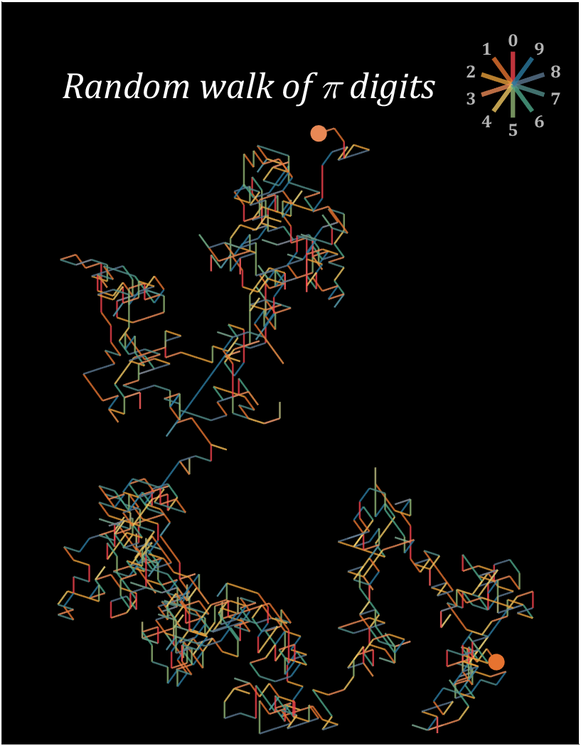
8 random walk
n=1200;
% 获取pi前n位小数
Pi=getPi(n);
CM=[239,65,75;230,115,48;229,158,57;232,136,85;239,199,97;
144,180,116;78,166,136;81,140,136;90,118,142;43,121,159]./255;
hold on
endPoint=[0,0];
t=linspace(0,2*pi,100);
T=linspace(0,2*pi,11)+pi/2;
fill(endPoint(1)+cos(t).*.5,endPoint(2)+sin(t).*.5,CM(Pi(1)+1,:),'EdgeColor','none')
for i=1:n
theta=T(Pi(i)+1);
plot(endPoint(1)+[0,cos(theta)],endPoint(2)+[0,sin(theta)],'Color',[CM(Pi(i)+1,:),.8],'LineWidth',1.2);
endPoint=endPoint+[cos(theta),sin(theta)];
end
fill(endPoint(1)+cos(t).*.5,endPoint(2)+sin(t).*.5,CM(Pi(n)+1,:),'EdgeColor','none')
% 图窗和坐标区域修饰
set(gcf,'Position',[200,100,820,820]);
ax=gca;
ax.XTick=[];
ax.YTick=[];
ax.Color=[0,0,0];
ax.DataAspectRatio=[1,1,1];
ax.XLim=[-30,5];
ax.YLim=[-5,40];
% 绘制图例
endPoint=[1,35];
for i=1:10
theta=T(i);
plot(endPoint(1)+[0,cos(theta).*2],endPoint(2)+[0,sin(theta).*2],'Color',[CM(i,:),.8],'LineWidth',3);
text(endPoint(1)+cos(theta).*2.7,endPoint(2)+sin(theta).*2.7,num2str(i-1),'Color',[1,1,1].*.7,...
'FontSize',12,'FontWeight','bold','FontName','Cambria','HorizontalAlignment','center')
end
text(-15,35,'Random walk of \pi digits','Color',[1,1,1],'FontName','Cambria',...
'HorizontalAlignment','center','FontSize',25,'FontAngle','italic')
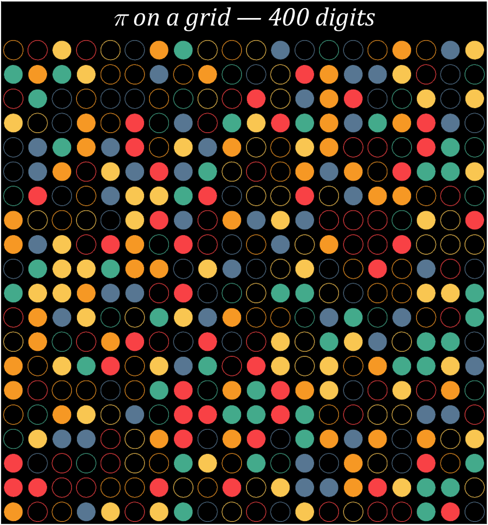
9 grid chart
Pi=[3,getPi(399)];
% 配色数据
CM=[248,65,69;246,152,36;249,198,81;67,170,139;87,118,146]./255;
% 绘制圆圈
hold on
t=linspace(0,2*pi,100);
x=cos(t).*.8.*.5;
y=sin(t).*.8.*.5;
for i=1:400
[col,row]=ind2sub([20,20],i);
if mod(Pi(i),2)==0
fill(x+col,y+row,CM(round((Pi(i)+1)/2),:),'LineWidth',1,'EdgeAlpha',.8)
else
fill(x+col,y+row,[0,0,0],'EdgeColor',CM(round((Pi(i)+1)/2),:),'LineWidth',1,'EdgeAlpha',.7)
end
end
text(10.5,-.4,'\pi on a grid — 400 digits','Color',[1,1,1],'FontName','Cambria',...
'HorizontalAlignment','center','FontSize',25,'FontAngle','italic')
% 图窗和坐标区域修饰
set(gcf,'Position',[200,100,820,820]);
ax=gca;
ax.YDir='reverse';
ax.XLim=[.5,20.5];
ax.YLim=[-1,20.5];
ax.XTick=[];
ax.YTick=[];
ax.Color=[0,0,0];
ax.DataAspectRatio=[1,1,1];
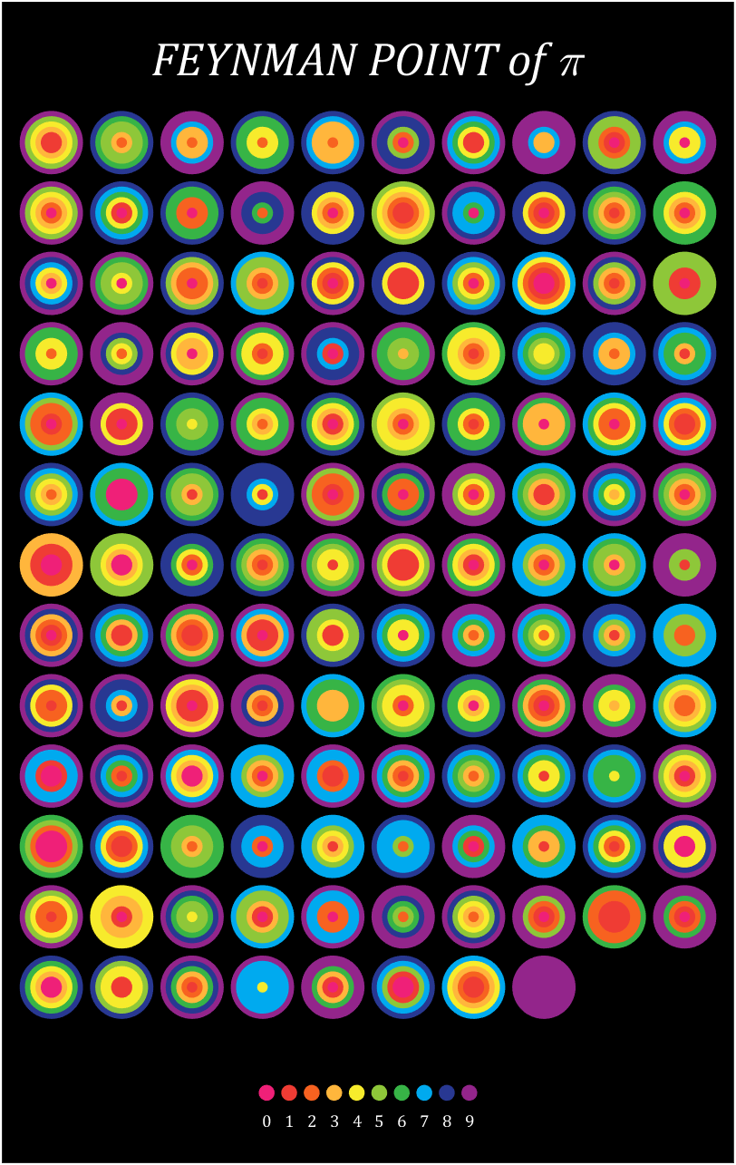
10 scale grid diagram
Let's still put the numbers in the form of circles, but the difference is that six numbers are grouped together, and the pure purple circle at the end is the six 9s that we are familiar with decimal places 762-767
Pi=[3,getPi(767)];
% 762-767
% 配色数据
CM=[239,32,120;239,60,52;247,98,32;255,182,60;247,235,44;
142,199,57;55,180,70;0,170,239;40,56,146;147,37,139]./255;
% 绘制圆圈
hold on
t=linspace(0,2*pi,100);
x=cos(t).*.9.*.5;
y=sin(t).*.9.*.5;
for i=1:6:length(Pi)
n=round((i-1)/6+1);
[col,row]=ind2sub([10,13],n);
tNum=Pi(i:i+5);
numNum=find([diff(sort(tNum)),1]);
numNum=[numNum(1),diff(numNum)];
cumNum=cumsum(numNum);
uniNum=unique(tNum);
for j=length(cumNum):-1:1
fill(x./6.*cumNum(j)+col,y./6.*cumNum(j)+row,CM(uniNum(j)+1,:),'EdgeColor','none')
end
end
% 绘制图例
for i=1:10
fill(x./4+5.5+(i-5.5)*.32,y./4+14.5,CM(i,:),'EdgeColor','none')
text(5.5+(i-5.5)*.32,14.9,num2str(i-1),'Color',[1,1,1],'FontSize',...
9,'FontName','Cambria','HorizontalAlignment','center')
end
text(5.5,-.2,'FEYNMAN POINT of \pi','Color',[1,1,1],'FontName','Cambria',...
'HorizontalAlignment','center','FontSize',25,'FontAngle','italic')
% 图窗和坐标区域修饰
set(gcf,'Position',[200,100,600,820]);
ax=gca;
ax.YDir='reverse';
ax.Position=[0,0,1,1];
ax.XLim=[.3,10.7];
ax.YLim=[-1,15.5];
ax.XTick=[];
ax.YTick=[];
ax.Color=[0,0,0];
ax.DataAspectRatio=[1,1,1];
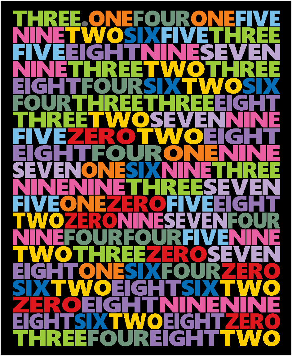
11 text chart

First, write a code to generate an image of each letter:
function getLogo
if ~exist('image','dir')
mkdir('image\')
end
logoSet=['.',char(65:90)];
for i=1:27
figure();
ax=gca;
ax.XLim=[-1,1];
ax.YLim=[-1,1];
ax.XColor='none';
ax.YColor='none';
ax.DataAspectRatio=[1,1,1];
logo=logoSet(i);
hold on
text(0,0,logo,'HorizontalAlignment','center','FontSize',320,'FontName','Segoe UI Black')
exportgraphics(ax,['image\',logo,'.png'])
close
end
dotPic=imread('image\..png');
newDotPic=uint8(ones([400,size(dotPic,2),3]).*255);
newDotPic(end-size(dotPic,1)+1:end,:,1)=dotPic(:,:,1);
newDotPic(end-size(dotPic,1)+1:end,:,2)=dotPic(:,:,2);
newDotPic(end-size(dotPic,1)+1:end,:,3)=dotPic(:,:,3);
imwrite(newDotPic,'image\..png')
S=20;
for i=1:27
logo=logoSet(i);
tPic=imread(['image\',logo,'.png']);
sz=size(tPic,[1,2]);
sz=round(sz./sz(1).*400);
tPic=imresize(tPic,sz);
tBox=uint8(255.*ones(size(tPic,[1,2])+S));
tBox(S+1:S+size(tPic,1),S+1:S+size(tPic,2))=tPic(:,:,1);
imwrite(cat(3,tBox,tBox,tBox),['image\',logo,'.png'])
end
end

Pi=[3,-1,getPi(150)];
CM=[109,110,113;224,25,33;244,126,26;253,207,2;154,203,57;111,150,124;
121,192,235;6,109,183;190,168,209;151,118,181;233,93,163]./255;
ST={'.','ZERO','ONE','TWO','THREE','FOUR','FIVE','SIX','SEVEN','EIGHT','NINE'};
n=1;
hold on
% 循环绘制字母
for i=1:20%:10
STList='';
NMList=[];
PicListR=uint8(zeros(400,0));
PicListG=uint8(zeros(400,0));
PicListB=uint8(zeros(400,0));
% PicListA=uint8(zeros(400,0));
for j=1:6
STList=[STList,ST{Pi(n)+2}];
NMList=[NMList,ones(size(ST{Pi(n)+2})).*(Pi(n)+2)];
n=n+1;
if length(STList)>15&&length(STList)+length(ST{Pi(n)+2})>20
break;
end
end
for k=1:length(STList)
tPic=imread(['image\',STList(k),'.png']);
% PicListA=[PicListA,tPic(:,:,1)];
PicListR=[PicListR,(255-tPic(:,:,1)).*CM(NMList(k),1)];
PicListG=[PicListG,(255-tPic(:,:,2)).*CM(NMList(k),2)];
PicListB=[PicListB,(255-tPic(:,:,3)).*CM(NMList(k),3)];
end
PicList=cat(3,PicListR,PicListG,PicListB);
image([-1200,1200],[0,150]-(i-1)*150,flipud(PicList))
end
% 图窗及坐标区域修饰
set(gcf,'Position',[200,100,600,820]);
ax=gca;
ax.DataAspectRatio=[1,1,1];
ax.XLim=[-1300,1300];
ax.Position=[0,0,1,1];
ax.XTick=[];
ax.YTick=[];
ax.Color=[0,0,0];
ax.YLim=[-19*150-80,230];
12 spiral chart
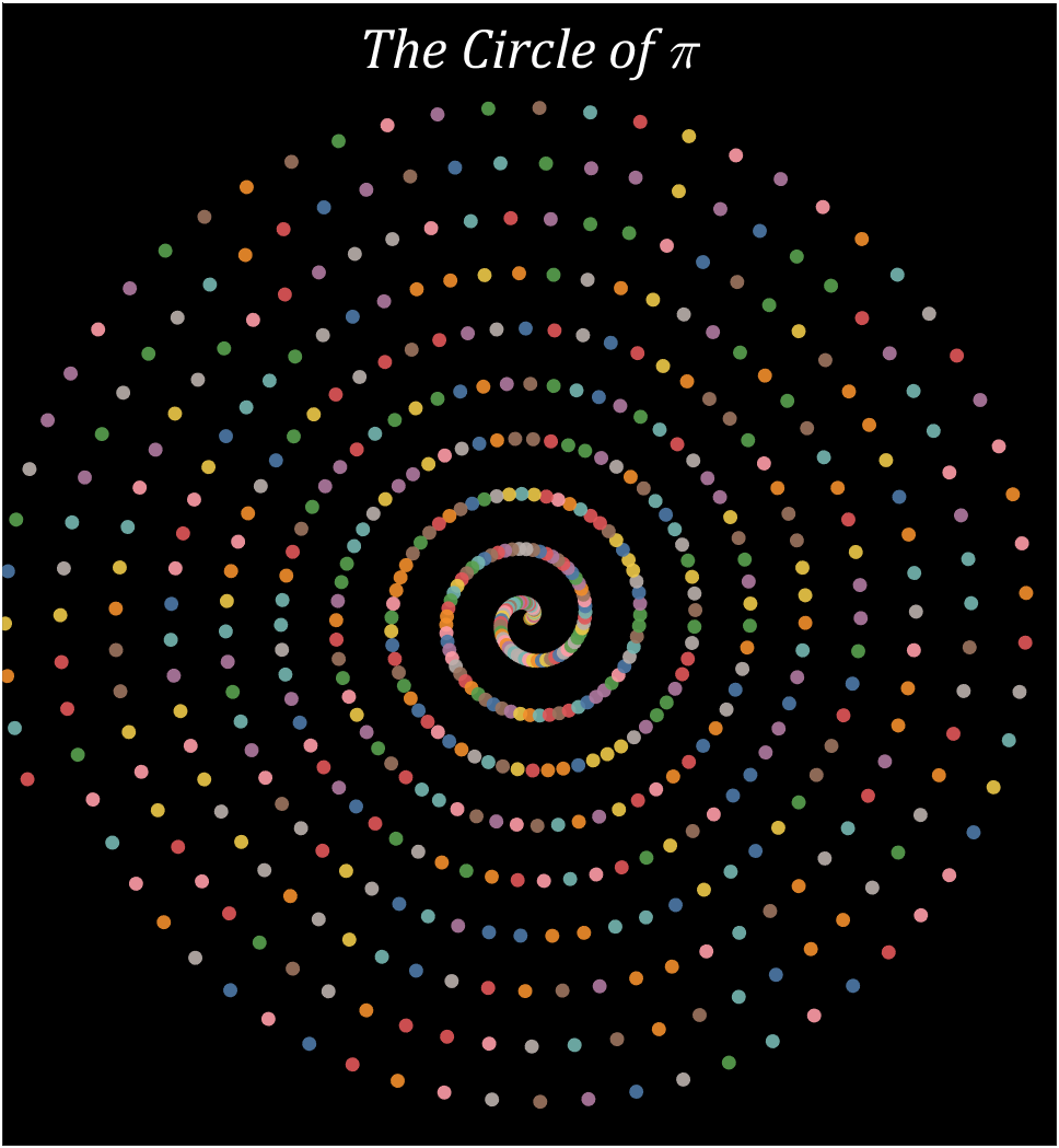
Pi=getPi(600);
% 配色列表
CM=[78,121,167;242,142,43;225,87,89;118,183,178;89,161,79;
237,201,72;176,122,161;255,157,167;156,117,95;186,176,172]./255;
% 绘制圆圈
hold on
t=linspace(0,2*pi,100);
x=cos(t).*.8;
y=sin(t).*.8;
for i=1:600
X=i.*cos(i./10)./10;
Y=i.*sin(i./10)./10;
fill(X+x,Y+y,CM(Pi(i)+1,:),'EdgeColor','none','FaceAlpha',.9)
end
text(0,65,'The Circle of \pi','Color',[1,1,1],'FontName','Cambria',...
'HorizontalAlignment','center','FontSize',25,'FontAngle','italic')
% 图窗和坐标区域修饰
set(gcf,'Position',[200,100,820,820]);
ax=gca;
ax.XLim=[-60,60];
ax.YLim=[-60,70];
ax.XTick=[];
ax.YTick=[];
ax.Color=[0,0,0];
ax.DataAspectRatio=[1,1,1];
13 Archimedean spiral diagram
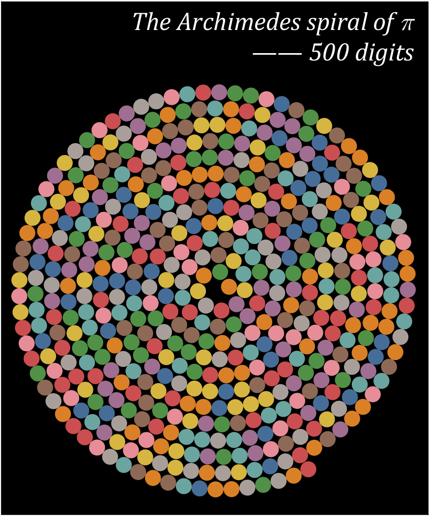
a=1;b=.227;
Pi=getPi(500);
% 配色列表
CM=[78,121,167;242,142,43;225,87,89;118,183,178;89,161,79;
237,201,72;176,122,161;255,157,167;156,117,95;186,176,172]./255;
% 绘制圆圈
hold on
T=0;R=1;
t=linspace(0,2*pi,100);
x=cos(t).*.7;
y=sin(t).*.7;
for i=1:500
X=R.*cos(T);Y=R.*sin(T);
fill(X+x,Y+y,CM(Pi(i)+1,:),'EdgeColor','none','FaceAlpha',.9)
T=T+1./R.*1.4;
R=a+b*T;
end
text(17.25,22,{'The Archimedes spiral of \pi';'—— 500 digits'},...
'Color',[1,1,1],'FontName','Cambria',...
'HorizontalAlignment','right','FontSize',25,'FontAngle','italic')
% 图窗和坐标区域修饰
set(gcf,'Position',[200,100,820,820]);
ax=gca;
ax.XLim=[-19,18.5];
ax.YLim=[-20,25];
ax.XTick=[];
ax.YTick=[];
ax.Color=[0,0,0];
ax.DataAspectRatio=[1,1,1];
14 proportional Archimedean spiral diagram
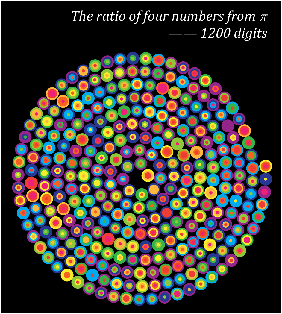
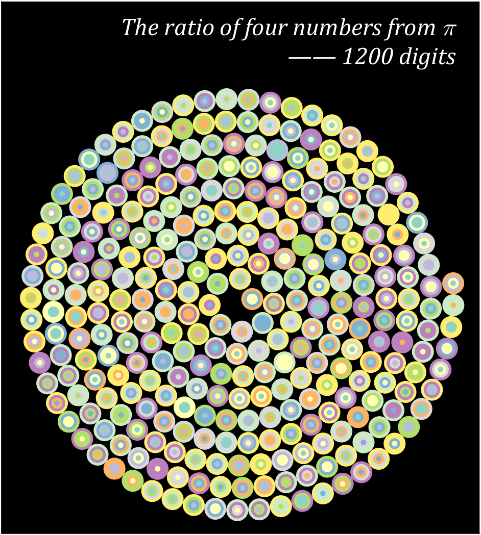
Pi=[3,getPi(1199)];
% 配色数据
CM=[239,32,120;239,60,52;247,98,32;255,182,60;247,235,44;
142,199,57;55,180,70;0,170,239;40,56,146;147,37,139]./255;
% CM=slanCM(184,10);
% 绘制圆圈
hold on
T=0;R=1;
t=linspace(0,2*pi,100);
x=cos(t).*.7;
y=sin(t).*.7;
for i=1:4:length(Pi)
X=R.*cos(T);Y=R.*sin(T);
tNum=Pi(i:i+3);
numNum=find([diff(sort(tNum)),1]);
numNum=[numNum(1),diff(numNum)];
cumNum=cumsum(numNum);
uniNum=unique(tNum);
for j=length(cumNum):-1:1
fill(x./4.*cumNum(j)+X,y./4.*cumNum(j)+Y,CM(uniNum(j)+1,:),'EdgeColor','none')
end
T=T+1./R.*1.4;
R=a+b*T;
end
text(14,16.5,{'The ratio of four numbers from \pi';'—— 1200 digits'},...
'Color',[1,1,1],'FontName','Cambria',...
'HorizontalAlignment','right','FontSize',23,'FontAngle','italic')
% 图窗和坐标区域修饰
set(gcf,'Position',[200,100,820,820]);
ax=gca;
ax.XLim=[-15,15.5];
ax.YLim=[-15,19];
ax.XTick=[];
ax.YTick=[];
ax.Color=[0,0,0];
ax.DataAspectRatio=[1,1,1];
15 graph
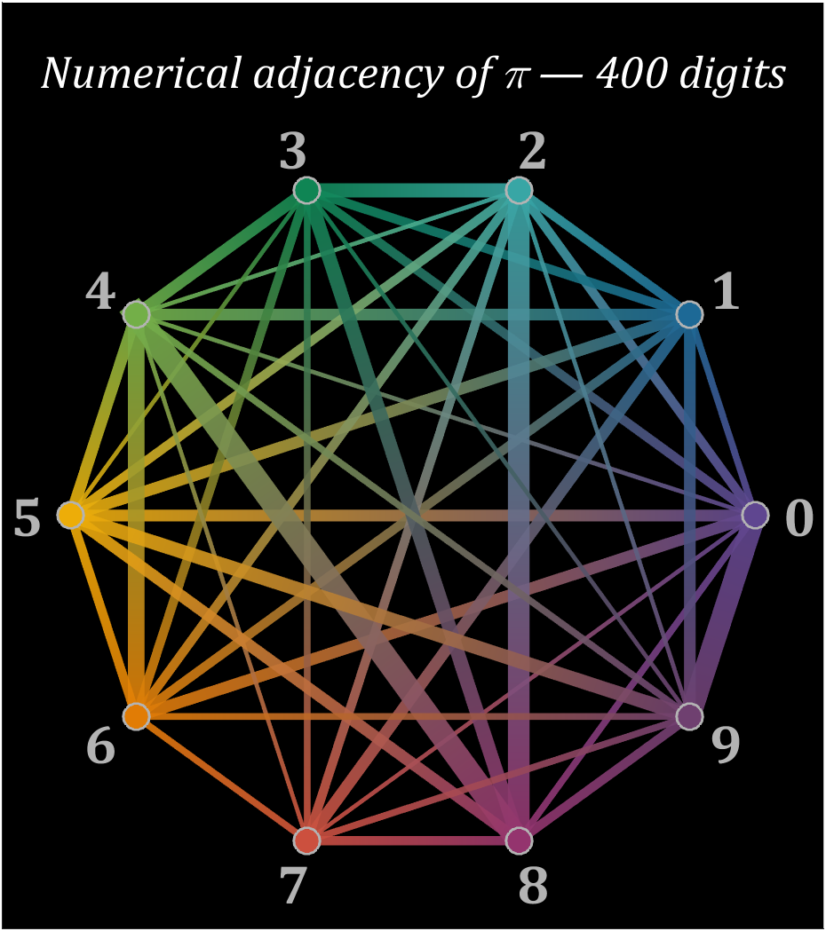
% 构建连接矩阵
corrMat=zeros(10,10);
Pi=getPi(401);
for i=1:400
corrMat(Pi(i)+1,Pi(i+1)+1)=corrMat(Pi(i)+1,Pi(i+1)+1)+1;
end
% 配色列表
colorList=[0.3725 0.2745 0.5647
0.1137 0.4118 0.5882
0.2196 0.6510 0.6471
0.0588 0.5216 0.3294
0.4510 0.6863 0.2824
0.9294 0.6784 0.0314
0.8824 0.4863 0.0196
0.8000 0.3137 0.2431
0.5804 0.2039 0.4314
0.4353 0.2510 0.4392];
t=linspace(0,2*pi,11);t=t(1:10)';
posXY=[cos(t),sin(t)];
maxWidth=max(corrMat(corrMat>0));
minWidth=min(corrMat(corrMat>0));
ttList=linspace(0,1,3)';
% 循环绘图
hold on
for i=1:size(corrMat,1)
for j=i+1:size(corrMat,2)
if corrMat(i,j)>0
tW=(corrMat(i,j)-minWidth)./(maxWidth-minWidth);
colorData=(1-ttList).*colorList(i,:)+ttList.*colorList(j,:);
CData(:,:,1)=colorData(:,1);
CData(:,:,2)=colorData(:,2);
CData(:,:,3)=colorData(:,3);
% 绘制连线
fill(linspace(posXY(i,1),posXY(j,1),3),...
linspace(posXY(i,2),posXY(j,2),3),[0,0,0],'LineWidth',tW.*12+1,...
'CData',CData,'EdgeColor','interp','EdgeAlpha',.7,'FaceAlpha',.7)
end
end
% 绘制圆点
scatter(posXY(i,1),posXY(i,2),200,'filled','LineWidth',1.2,...
'MarkerFaceColor',colorList(i,:),'MarkerEdgeColor',[.7,.7,.7]);
text(posXY(i,1).*1.13,posXY(i,2).*1.13,num2str(i-1),'Color',[1,1,1].*.7,...
'FontSize',30,'FontWeight','bold','FontName','Cambria','HorizontalAlignment','center')
end
text(0,1.3,'Numerical adjacency of \pi — 400 digits','Color',[1,1,1],'FontName','Cambria',...
'HorizontalAlignment','center','FontSize',25,'FontAngle','italic')
% 图窗和坐标区域修饰
set(gcf,'Position',[200,100,820,820]);
ax=gca;
ax.XLim=[-1.2,1.2];
ax.YLim=[-1.21,1.5];
ax.XTick=[];
ax.YTick=[];
ax.Color=[0,0,0];
ax.DataAspectRatio=[1,1,1];
16 circos chart
Need to use this tool:
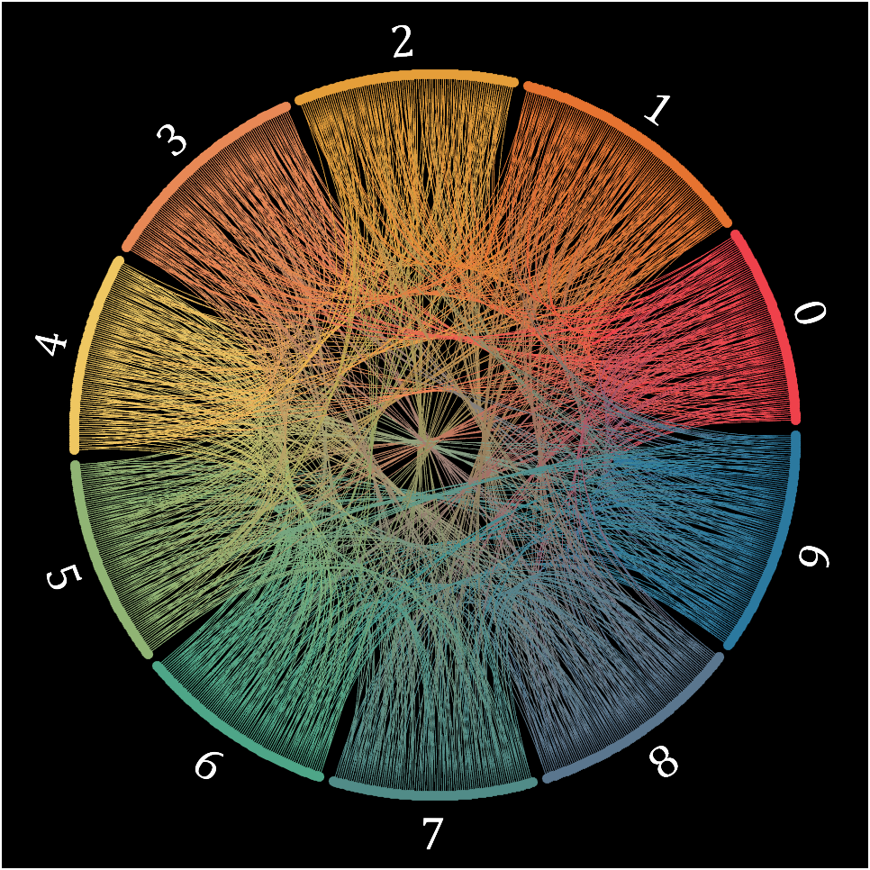
Class=getPi(1001)+1;
Data=diag(ones(1,1000),-1);
className={'0','1','2','3','4','5','6','7','8','9'};
colorOrder=[239,65,75;230,115,48;229,158,57;232,136,85;239,199,97;
144,180,116;78,166,136;81,140,136;90,118,142;43,121,159]./255;
CC=circosChart(Data,Class,'ClassName',className,'ColorOrder',colorOrder);
CC=CC.draw();
ax=gca;
ax.Color=[0,0,0];
CC.setClassLabel('Color',[1,1,1],'FontSize',25,'FontName','Cambria')
CC.setLine('LineWidth',.7)
YOU CAN GET ALL CODE HERE:
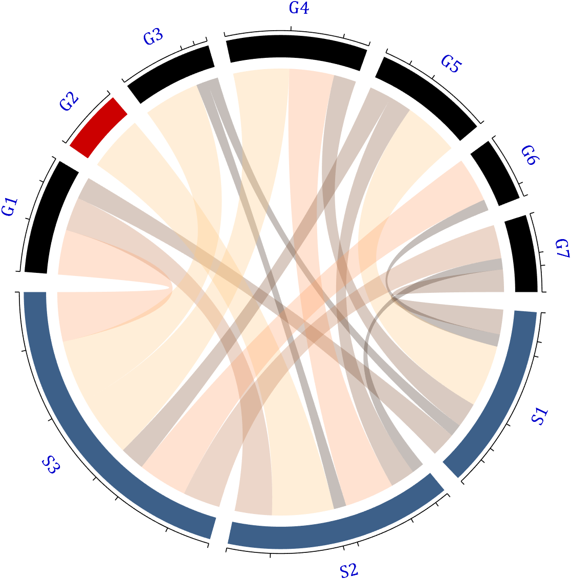
Chord diagrams are very common in Python and R, but there are no related functions in MATLAB before. It is not easy to draw chord diagrams of the same quality as R language, But I created a MATLAB tool that could almost do it.
↓ ↓ ↓ ↓ ↓ ↓ ↓ ↓ ↓ ↓
↑ ↑ ↑ ↑ ↑ ↑ ↑ ↑ ↑ ↑
Here is the help document:
1 Data Format
The data requirement is a numerical matrix with all values greater than or equal to 0, or a table array, or a numerical matrix and cell array for names. First, give an example of a numerical matrix:
1.1 Numerical Matrix
dataMat=randi([0,5],[5,4]);
% 绘图(draw)
CC=chordChart(dataMat);
CC=CC.draw();
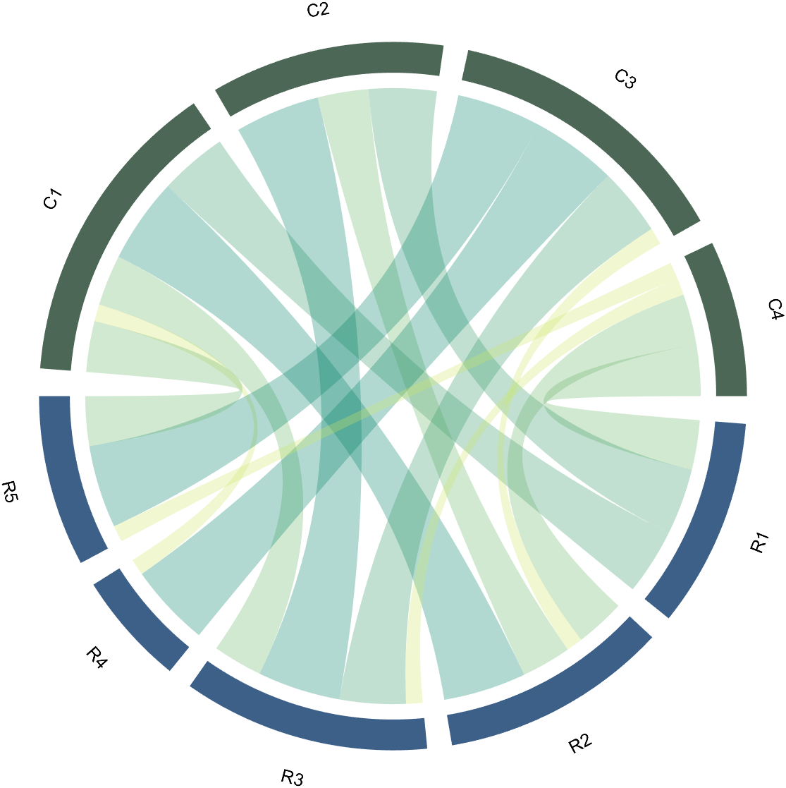
Since each object is not named, it will be automatically named Rn and Cn
1.2 Numerical Matrix and Cell Array for Names
dataMat=[2 0 1 2 5 1 2;
3 5 1 4 2 0 1;
4 0 5 5 2 4 3];
colName={'G1','G2','G3','G4','G5','G6','G7'};
rowName={'S1','S2','S3'};
CC=chordChart(dataMat,'rowName',rowName,'colName',colName);
CC=CC.draw();

RowName should be the same size as the rows of the matrix
ColName should be the same size as the columns of the matrix
For this example, if the value in the second row and third column is 1, it indicates that there is an energy flow from S2 to G3, and a chord with a width of 1 is needed between these two.
1.3 Table Array
A table array in the following format is required:
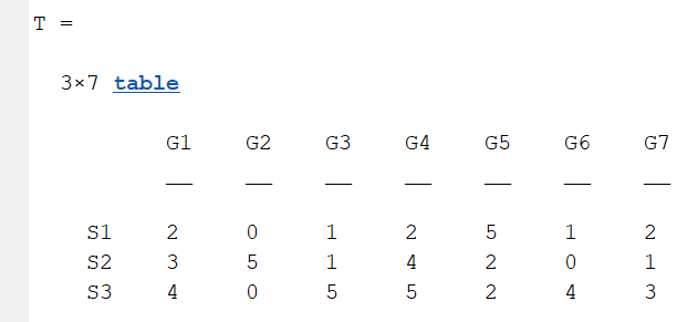
2 Decorate Chord
2.1 Batch modification of chords
Batch modification of chords can be done using the setChordProp function, and all properties of the Patch object can be modified. For example, modifying the color of the string, edge color, edge line sstyle, etc.:
CC.setChordProp('EdgeColor',[.3,.3,.3],'LineStyle','--',...
'LineWidth',.1,'FaceColor',[.3,.3,.3])
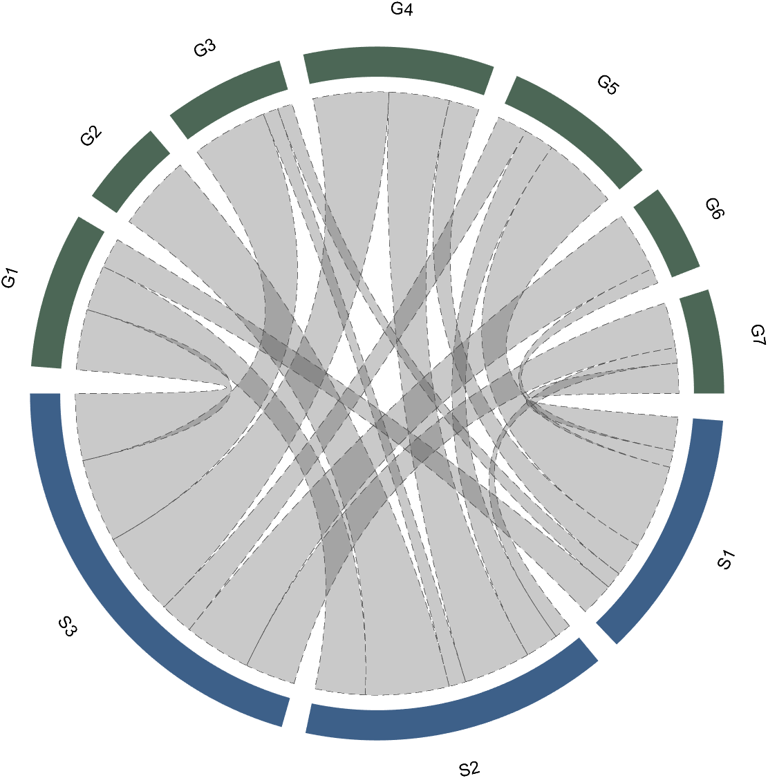
2.2 Individual Modification of Chord
The individual modification of chord can be done using the setChordMN function, where the values of m and n correspond exactly to the rows and columns of the original numerical matrix. For example, changing the color of the strings flowing from S2 to G4 to red:
CC.setChordMN(2,4,'FaceColor',[1,0,0])
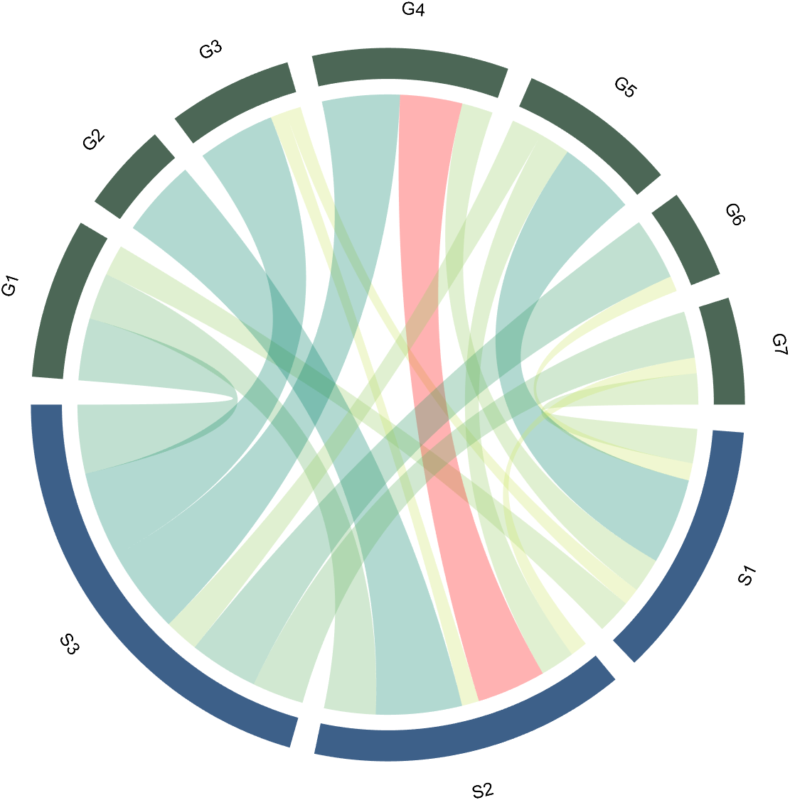
2.3 Color Mapping of Chords
Just use function colormap to do so:
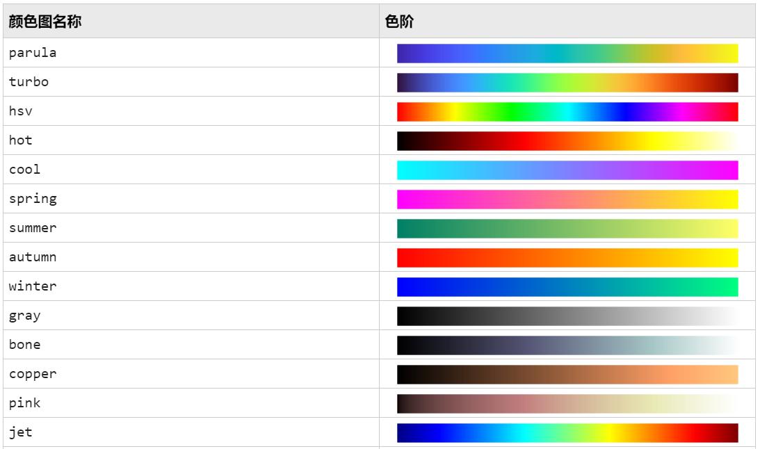
% version 1.7.0更新
% 可使用colormap函数直接修改颜色
% Colors can be adjusted directly using the function colormap(demo4)
colormap(flipud(pink))
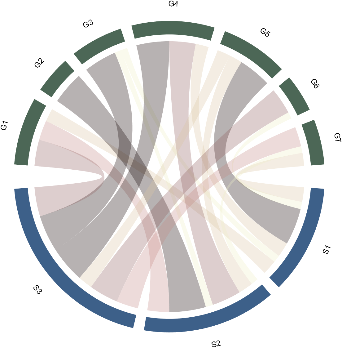
3 Arc Shaped Block Decoration
3.1 Batch Decoration of Arc-Shaped Blocks
use:
- setSquareT_Prop
- setSquareF_Prop
to modify the upper and lower blocks separately, and all attributes of the Patch object can be modified. For example, batch modify the upper blocks (change to black):
CC.setSquareT_Prop('FaceColor',[0,0,0])
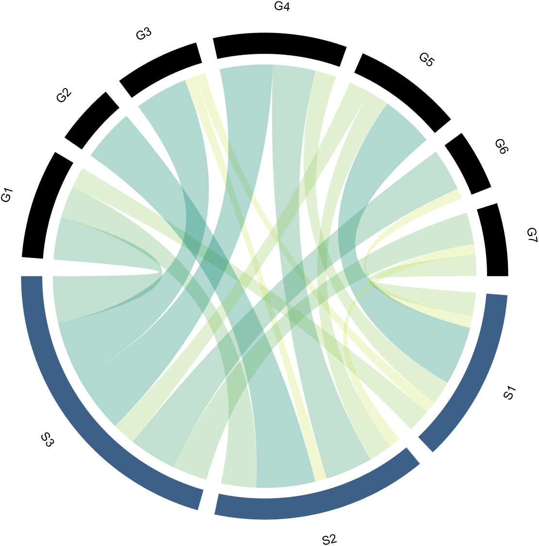
3.2 Arc-Shaped Blocks Individually Decoration
use:
- setSquareT_N
- setSquareF_N
to modify the upper and lower blocks separately. For example, modify the second block above separately (changed to red):
CC.setSquareT_N(2,'FaceColor',[.8,0,0])
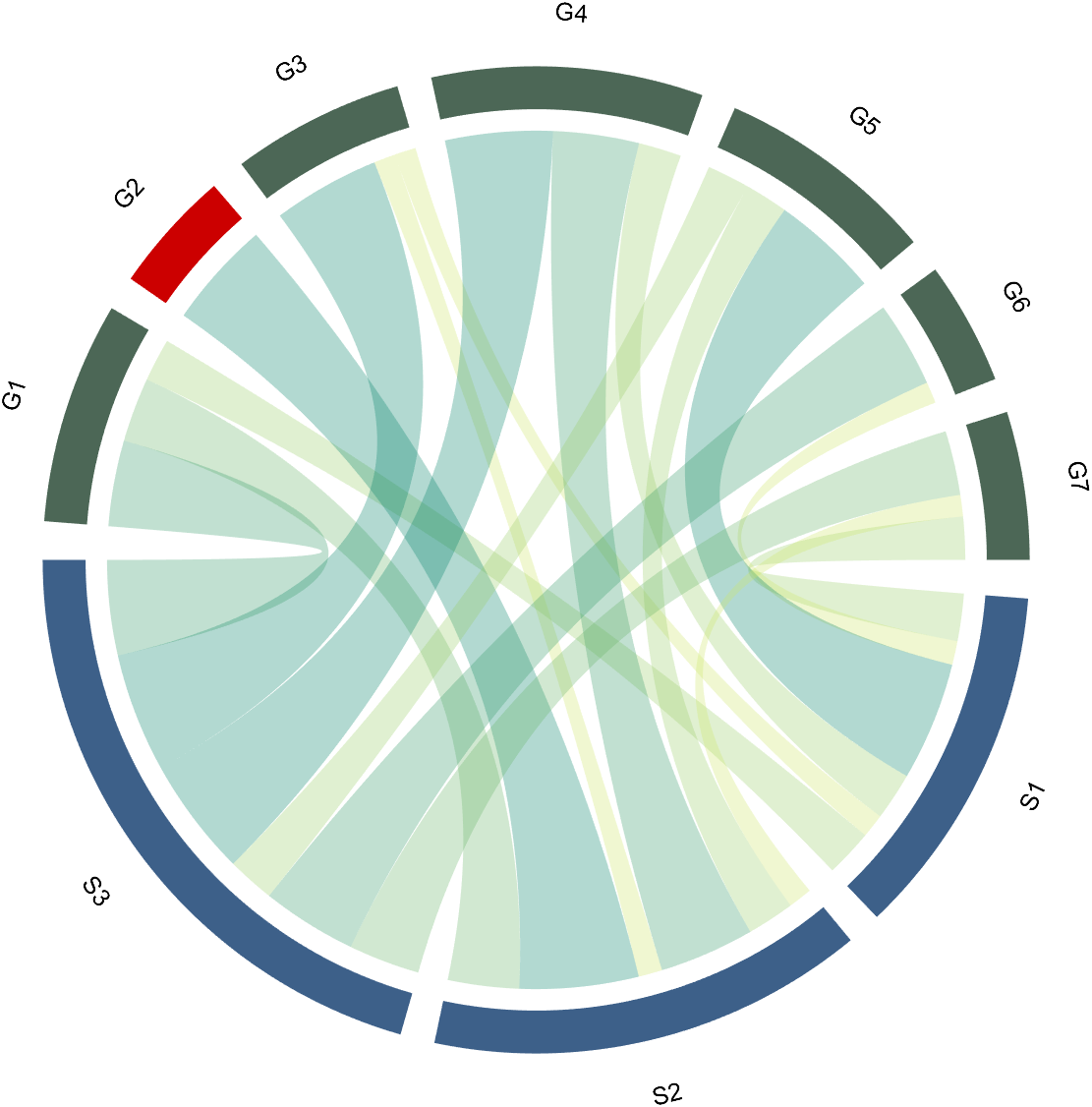
4 Font Adjustment
Use the setFont function to adjust the font, and all properties of the text object can be modified. For example, changing the font size, font, and color of the text:
CC.setFont('FontSize',25,'FontName','Cambria','Color',[0,0,.8])
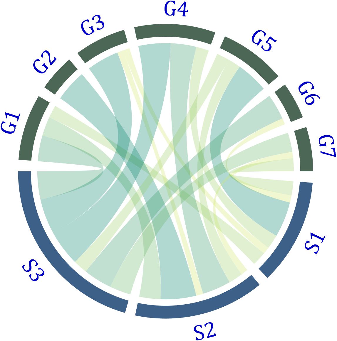
5 Show and Hide Ticks
Usage:
CC.tickState('on')
% CC.tickState('off')
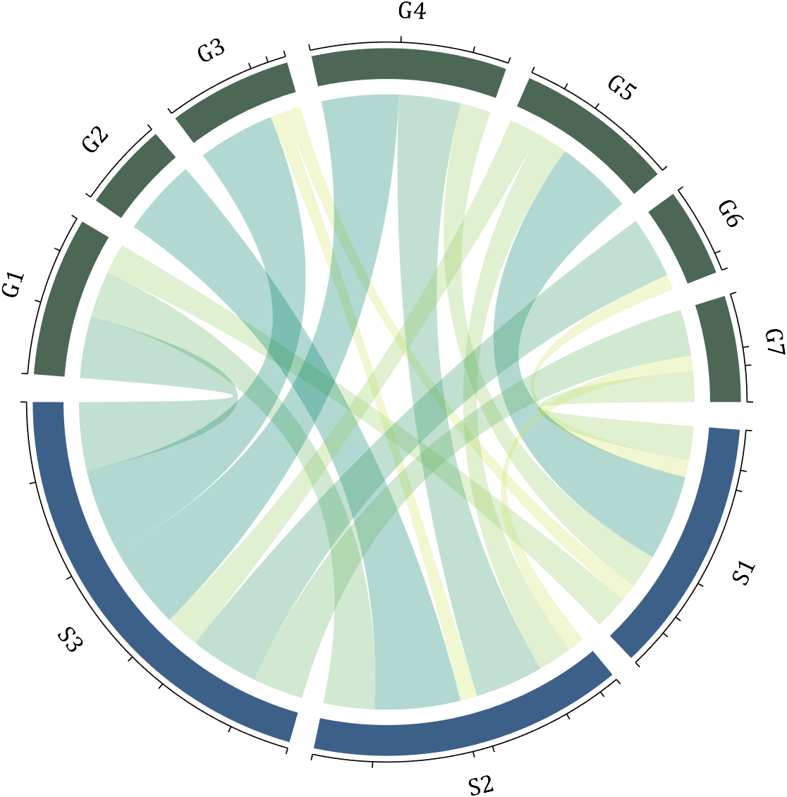
6 Attribute 'Sep' with Adjustable Square Spacing
If the matrix size is large, the drawing will be out of scale:
dataMat=randi([0,1],[20,10]);
CC=chordChart(dataMat);
CC=CC.draw();
% CC.tickState('on')
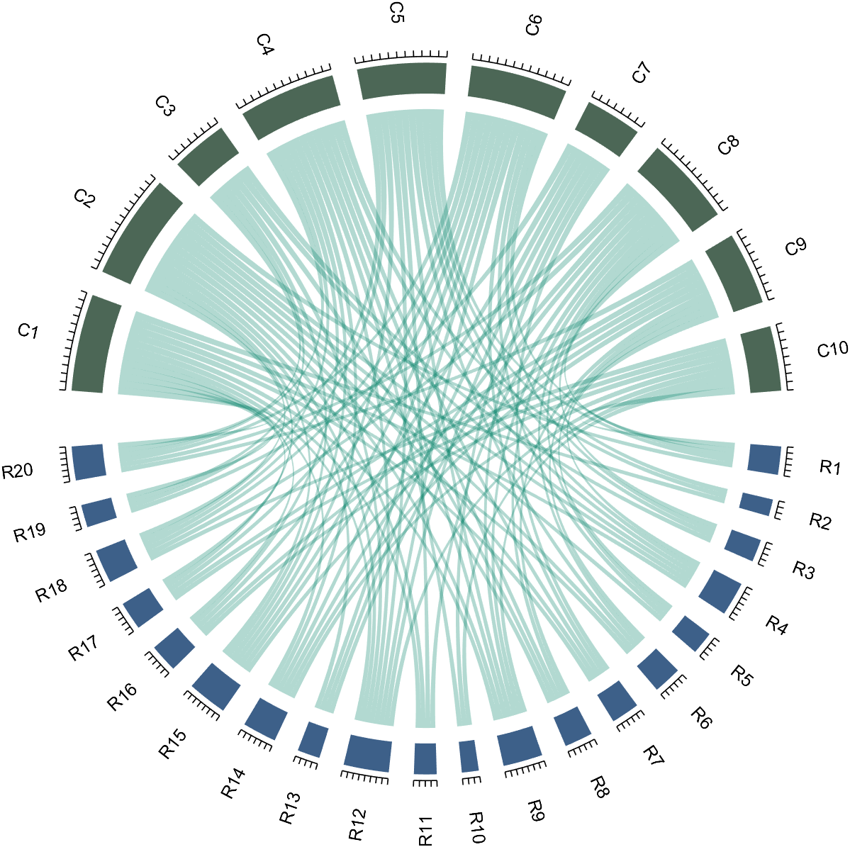
We can modify its Sep attribute:
dataMat=randi([0,1],[20,10]);
% use Sep to decrease space (separation)
% 使用 sep 减小空隙
CC=chordChart(dataMat,'Sep',1/120);
CC=CC.draw();
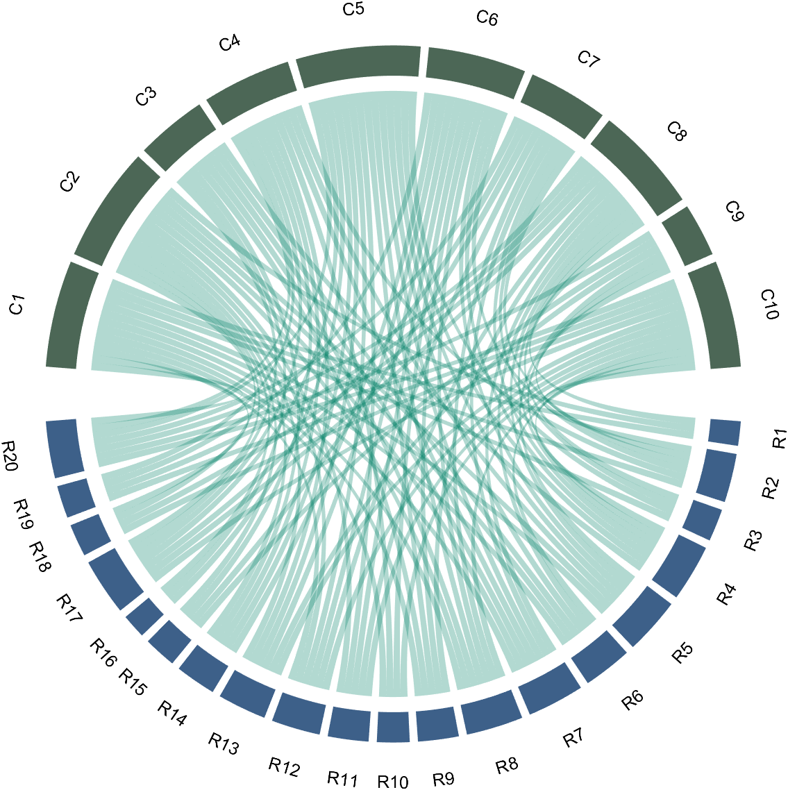
7 Modify Text Direction
dataMat=randi([0,1],[20,10]);
% use Sep to decrease space (separation)
% 使用 sep 减小空隙
CC=chordChart(dataMat,'Sep',1/120);
CC=CC.draw();
CC.tickState('on')
% version 1.7.0更新
% 函数labelRatato用来旋转标签
% The function labelRatato is used to rotate the label
CC.labelRotate('on')
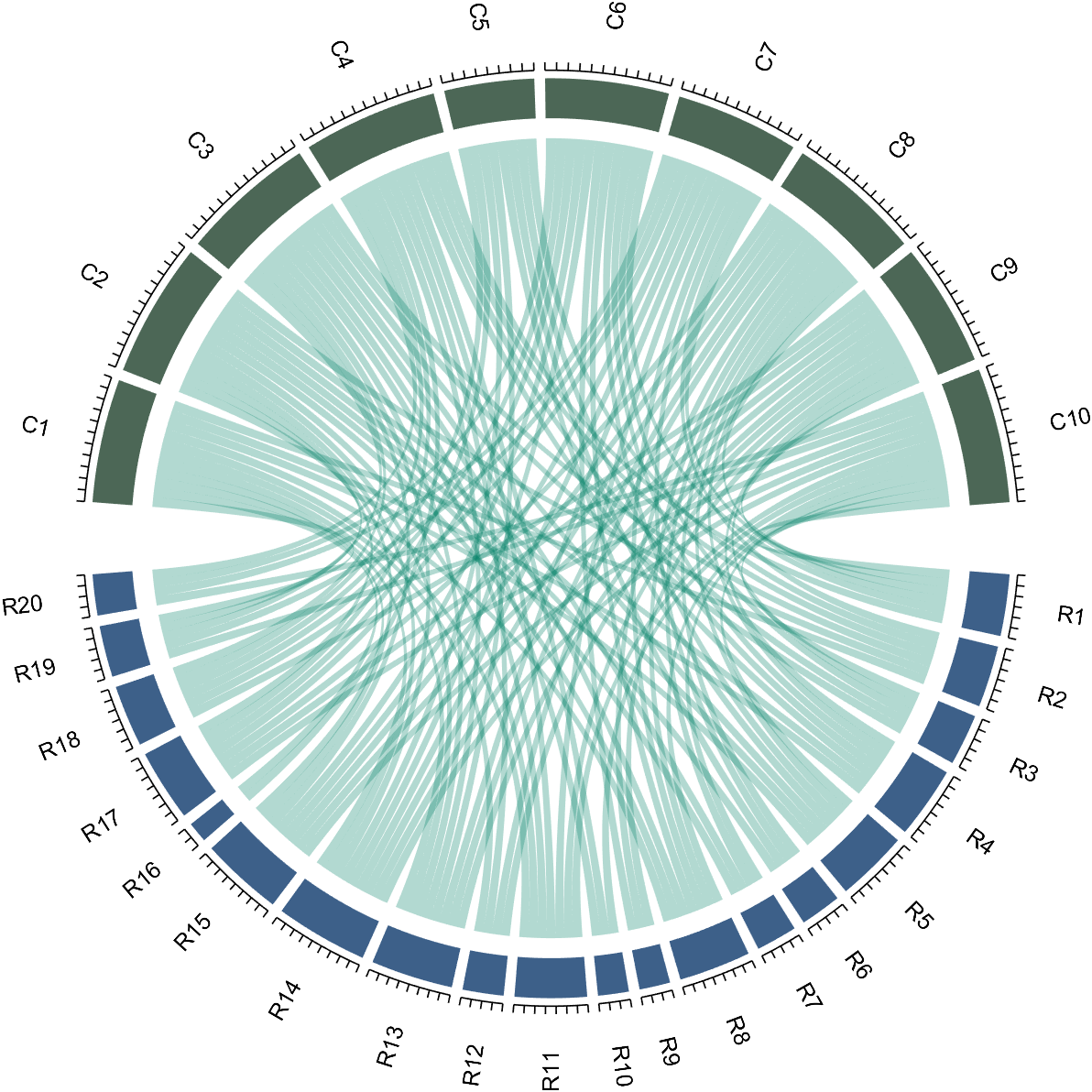
8 Add Tick Labels
dataMat=[2 0 1 2 5 1 2;
3 5 1 4 2 0 1;
4 0 5 5 2 4 3];
colName={'G1','G2','G3','G4','G5','G6','G7'};
rowName={'S1','S2','S3'};
CC=chordChart(dataMat,'rowName',rowName,'colName',colName);
CC=CC.draw();
CC.setFont('FontSize',17,'FontName','Cambria')
% 显示刻度和数值
% Displays scales and numeric values
CC.tickState('on')
CC.tickLabelState('on')
% 调节标签半径
% Adjustable Label radius
CC.setLabelRadius(1.3);
% figure()
% dataMat=[2 0 1 2 5 1 2;
% 3 5 1 4 2 0 1;
% 4 0 5 5 2 4 3];
% dataMat=dataMat+rand(3,7);
% dataMat(dataMat<1)=0;
%
% CC=chordChart(dataMat,'rowName',rowName,'colName',colName);
% CC=CC.draw();
% CC.setFont('FontSize',17,'FontName','Cambria')
%
% % 显示刻度和数值
% % Displays scales and numeric values
% CC.tickState('on')
% CC.tickLabelState('on')
%
% % 调节标签半径
% % Adjustable Label radius
% CC.setLabelRadius(1.4);
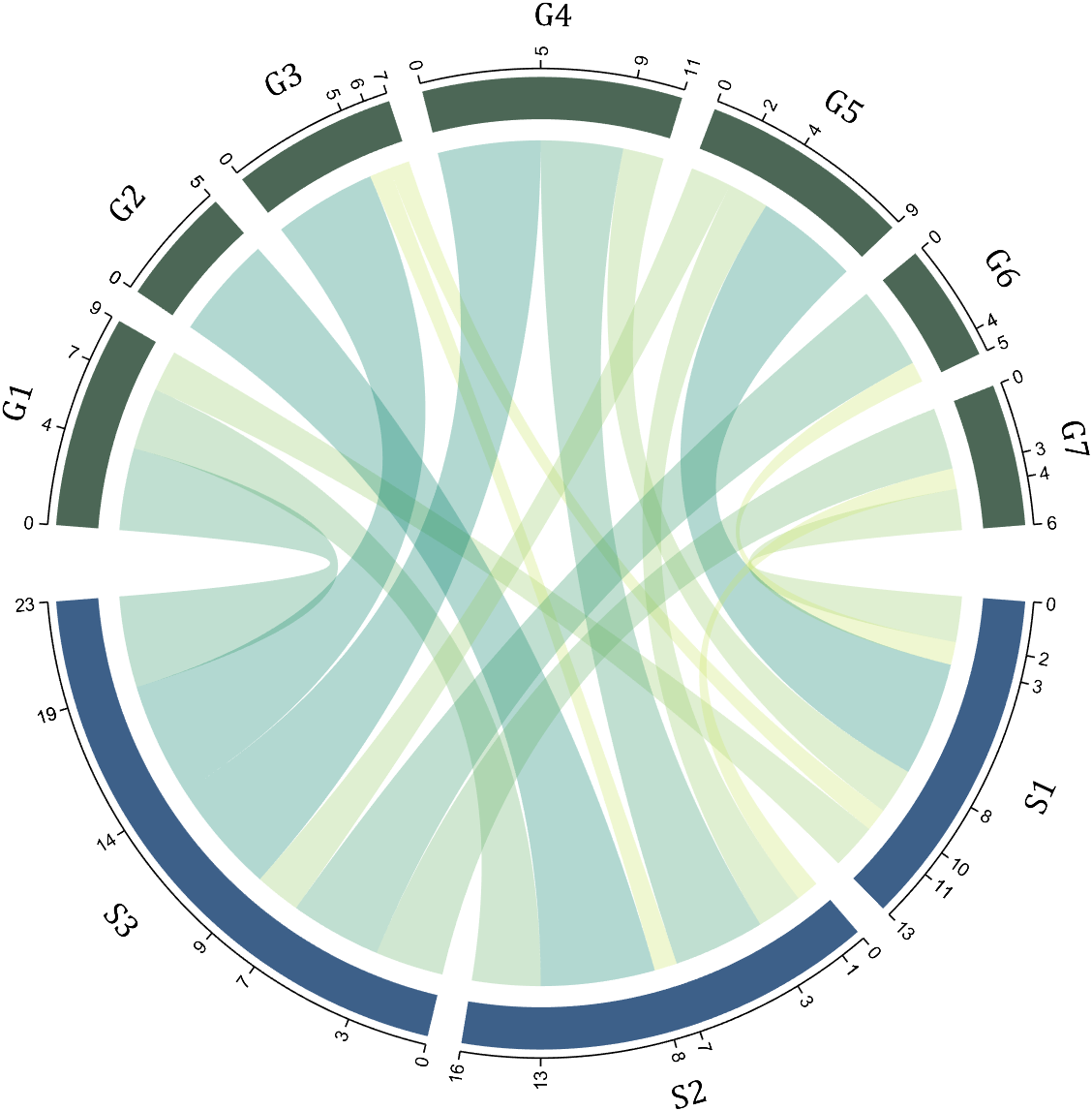
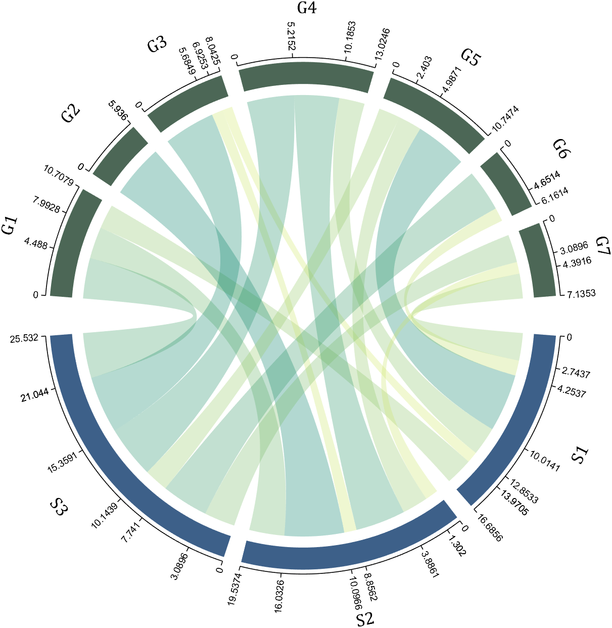
9 Custom Tick Label Format
A function handle is required to input numeric output strings. The format can be set through the setTickLabelFormat function, such as Scientific notation:
dataMat=[2 0 1 2 5 1 2;
3 5 1 4 2 0 1;
4 0 5 5 2 4 3];
dataMat=dataMat+rand(3,7);
dataMat(dataMat<1)=0;
dataMat=dataMat.*1000;
CC=chordChart(dataMat);
CC=CC.draw();
CC.setFont('FontSize',17,'FontName','Cambria')
% 显示刻度和数值
% Displays scales and numeric values
CC.tickState('on')
CC.tickLabelState('on')
% 调节标签半径
% Adjustable Label radius
CC.setLabelRadius(1.4);
% 调整数值字符串格式
% Adjust numeric string format
CC.setTickLabelFormat(@(x)sprintf('%0.1e',x))
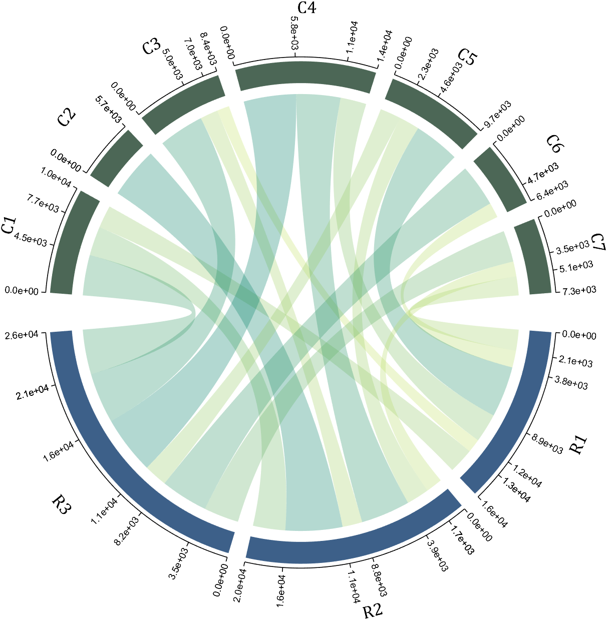
10 A Demo
rng(2)
dataMat=randi([1,7],[11,5]);
colName={'Fly','Beetle','Leaf','Soil','Waxberry'};
rowName={'Bartomella','Bradyrhizobium','Dysgomonas','Enterococcus',...
'Lactococcus','norank','others','Pseudomonas','uncultured',...
'Vibrionimonas','Wolbachia'};
CC=chordChart(dataMat,'rowName',rowName,'colName',colName,'Sep',1/80);
CC=CC.draw();
% 修改上方方块颜色(Modify the color of the blocks above)
CListT=[0.7765 0.8118 0.5216;0.4431 0.4706 0.3843;0.5804 0.2275 0.4549;
0.4471 0.4039 0.6745;0.0157 0 0 ];
for i=1:5
CC.setSquareT_N(i,'FaceColor',CListT(i,:))
end
% 修改下方方块颜色(Modify the color of the blocks below)
CListF=[0.5843 0.6863 0.7843;0.1098 0.1647 0.3255;0.0902 0.1608 0.5373;
0.6314 0.7961 0.2118;0.0392 0.2078 0.1059;0.0157 0 0 ;
0.8549 0.9294 0.8745;0.3882 0.3255 0.4078;0.5020 0.7216 0.3843;
0.0902 0.1843 0.1804;0.8196 0.2314 0.0706];
for i=1:11
CC.setSquareF_N(i,'FaceColor',CListF(i,:))
end
% 修改弦颜色(Modify chord color)
for i=1:5
for j=1:11
CC.setChordMN(j,i,'FaceColor',CListT(i,:),'FaceAlpha',.5)
end
end
CC.tickState('on')
CC.labelRotate('on')
CC.setFont('FontSize',17,'FontName','Cambria')
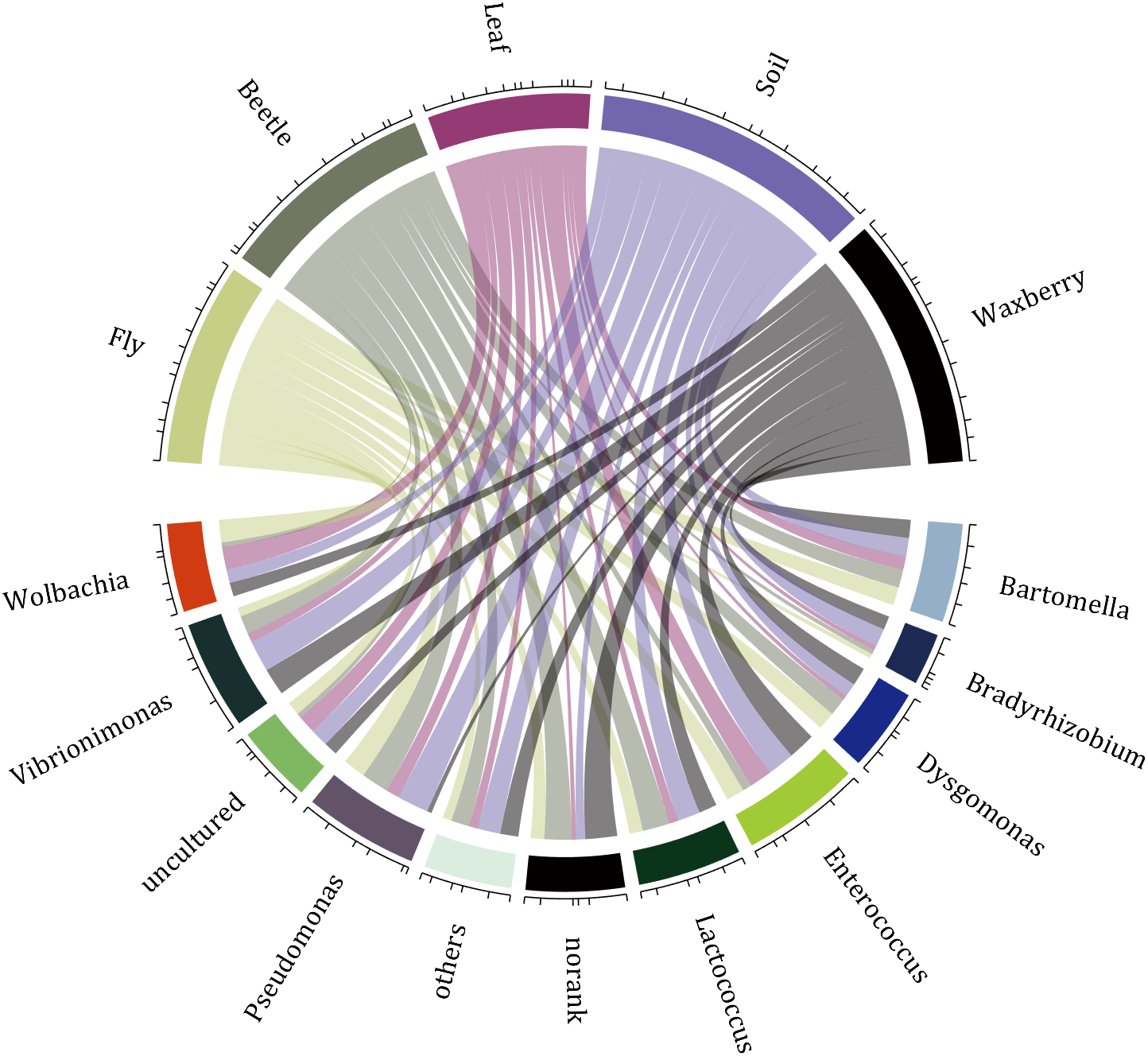
Hope to have your Reviews and Stars!!!
↓ ↓ ↓ ↓ ↓ ↓ ↓ ↓ ↓ ↓
↑ ↑ ↑ ↑ ↑ ↑ ↑ ↑ ↑ ↑
Most of my projects are the tension between what exists and what I must create to make the project work. The more I leverage what exists, the faster I can complete my project in a shorter amount of time. I often find out later in the process that a MATLAB function already exists and has existed for 10 releases. The faster that I discover built-in functions, the faster I can get to the new stuff that I have to invent.
I asked the AI Chat Playground why to use MATLAB's builtin functions and I got some interesting ideas. What are your thoughts?
AI Chat Playground:
- Efficiency and Performance: MATLAB's built-in functions are highly optimized for performance. They are written in optimized and compiled languages like C or C++, which means they run faster than equivalent functions written directly in MATLAB language. When you use these functions, your code can execute more efficiently, which is especially beneficial for handling large datasets or complex mathematical computations.
- Reliability and Stability: Built-in functions have been rigorously tested and debugged by the developers at MathWorks (the company behind MATLAB). They are less likely to contain errors compared to custom-written code, which means you can rely on them to produce accurate and consistent results.
- Ease of Use: Built-in functions are designed to be user-friendly, with clear documentation and support materials available. This can make it easier to perform complex operations without needing a deep understanding of the underlying algorithms. It also reduces the amount of code you need to write and debug, saving time and reducing the potential for errors.
- Compatibility: Built-in functions are updated alongside MATLAB itself, ensuring compatibility with new features and versions of the software. Using built-in functions can help ensure that your code continues to work correctly as MATLAB evolves.
- Advanced Features: MATLAB’s built-in functions often include advanced features and options that are not readily available or would be difficult to implement on your own. For example, MATLAB’s mathematical functions can handle a wide range of special cases and data types, providing more flexibility than custom implementations.
- Community and Support: Using built-in functions means you're working with standard tools recognized by the MATLAB community. This can make it easier to get help from other users or from MathWorks support, as more people will be familiar with the functionality and potential issues of these functions.
您也可以从以下列表中选择网站:
美洲
- América Latina (Español)
- Canada (English)
- United States (English)
欧洲
- Belgium (English)
- Denmark (English)
- Deutschland (Deutsch)
- España (Español)
- Finland (English)
- France (Français)
- Ireland (English)
- Italia (Italiano)
- Luxembourg (English)
- Netherlands (English)
- Norway (English)
- Österreich (Deutsch)
- Portugal (English)
- Sweden (English)
- Switzerland
- United Kingdom(English)
亚太
- Australia (English)
- India (English)
- New Zealand (English)
- 中国
- 日本Japanese (日本語)
- 한국Korean (한국어)