主要内容
Results for
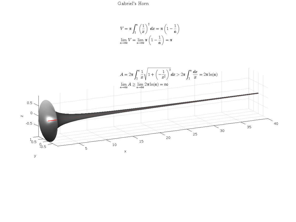
Gabriel's horn is a shape with the paradoxical property that it has infinite surface area, but a finite volume.
Gabriel’s horn is formed by taking the graph of  with the domain
  and rotating it in three dimensions about the
  axis.
axis.
There is a standard formula for calculating the volume of this shape, for a general function  .Wwe will just state that the volume of the
  solid between a and b is:
The surface area of the solid is given by:
One other thing we need to consider is that we are trying to find the value of these integrals between 1 and ∞. An integral with a limit of infinity is called an improper integral and we can't evaluate it simply by plugging the value infinity into the normal equation for a definite integral. Instead, we must first calculate the definite integral up to some finite limit b and then calculate the limit of the result as b tends to ∞:
Volume
We can calculate the horn's volume using the volume integral above, so
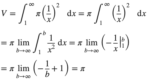
The total volume of this infinitely long trumpet isπ.
Surface Area
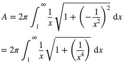
To determine the surface area, we first need the function’s derivative:
Now plug it into the surface area formula and we have:
This is an improper integral and it's hard to evaluate, but since in our interval 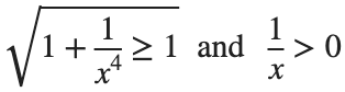
So, we have :
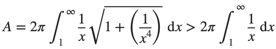
Now,we evaluate this last integral
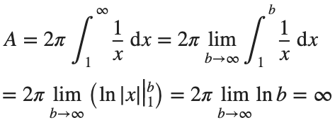
So the surface are is infinite.
% Define the function for Gabriel's Horn
gabriels_horn = @(x) 1 ./ x;
% Create a range of x values
x = linspace(1, 40, 4000); % Increase the number of points for better accuracy
y = gabriels_horn(x);
% Create the meshgrid
theta = linspace(0, 2 * pi, 6000); % Increase theta points for a smoother surface
[X, T] = meshgrid(x, theta);
Y = gabriels_horn(X) .* cos(T);
Z = gabriels_horn(X) .* sin(T);
% Plot the surface of Gabriel's Horn
figure('Position', [200, 100, 1200, 900]);
surf(X, Y, Z, 'EdgeColor', 'none', 'FaceAlpha', 0.9);
hold on;
% Plot the central axis
plot3(x, zeros(size(x)), zeros(size(x)), 'r', 'LineWidth', 2);
% Set labels
xlabel('x');
ylabel('y');
zlabel('z');
% Adjust colormap and axis properties
colormap('gray');
shading interp; % Smooth shading
% Adjust the view
view(3);
axis tight;
grid on;
% Add formulas as text annotations
dim1 = [0.4 0.7 0.3 0.2];
annotation('textbox',dim1,'String',{'$$V = \pi \int_{1}^{a} \left( \frac{1}{x} \right)^2 dx = \pi \left( 1 - \frac{1}{a} \right)$$', ...
'', ... % Add an empty line for larger gap
'$$\lim_{a \to \infty} V = \lim_{a \to \infty} \pi \left( 1 - \frac{1}{a} \right) = \pi$$'}, ...
'Interpreter','latex','FontSize',12, 'EdgeColor','none', 'FitBoxToText', 'on');
dim2 = [0.4 0.5 0.3 0.2];
annotation('textbox',dim2,'String',{'$$A = 2\pi \int_{1}^{a} \frac{1}{x} \sqrt{1 + \left( -\frac{1}{x^2} \right)^2} dx > 2\pi \int_{1}^{a} \frac{dx}{x} = 2\pi \ln(a)$$', ...
'', ... % Add an empty line for larger gap
'$$\lim_{a \to \infty} A \geq \lim_{a \to \infty} 2\pi \ln(a) = \infty$$'}, ...
'Interpreter','latex','FontSize',12, 'EdgeColor','none', 'FitBoxToText', 'on');
% Add Gabriel's Horn label
dim3 = [0.3 0.9 0.3 0.1];
annotation('textbox',dim3,'String','Gabriel''s Horn', ...
'Interpreter','latex','FontSize',14, 'EdgeColor','none', 'HorizontalAlignment', 'center');
hold off
daspect([3.5 1 1]) % daspect([x y z])
view(-27, 15)
lightangle(-50,0)
lighting('gouraud')
The properties of this figure were first studied by Italian physicist and mathematician Evangelista Torricelli in the 17th century.
Acknowledgment
I would like to express my sincere gratitude to all those who have supported and inspired me throughout this project.
First and foremost, I would like to thank the mathematician and my esteemed colleague, Stavros Tsalapatis, for inspiring me with the fascinating subject of Gabriel's Horn.
I am also deeply thankful to Mr. @Star Strider for his invaluable assistance in completing the final code.
References:
When it comes to MOS tube burnout, it is usually because it is not working in the SOA workspace, and there is also a case where the MOS tube is overcurrent.
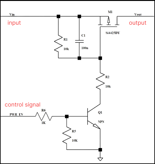
For example, the maximum allowable current of the PMOS transistor in this circuit is 50A, and the maximum current reaches 80+ at the moment when the MOS transistor is turned on, then the current is very large.
At this time, the PMOS is over-specified, and we can see on the SOA curve that it is not working in the SOA range, which will cause the PMOS to be damaged.
So what if you choose a higher current PMOS? Of course you can, but the cost will be higher.
We can choose to adjust the peripheral resistance or capacitor to make the PMOS turn on more slowly, so that the current can be lowered.
For example, when adjusting R1, R2, and the jumper capacitance between gs, when Cgs is adjusted to 1uF, The Ids are only 40A max, which is fine in terms of current, and meets the 80% derating.
(50 amps * 0.8 = 40 amps).
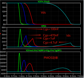
Next, let’s look at the power, from the SOA curve, the opening time of the MOS tube is about 1ms, and the maximum power at this time is 280W.
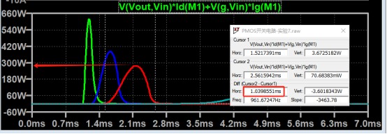
The normal thermal resistance of the chip is 50°C/W, and the maximum junction temperature can be 302°F.
Assuming the ambient temperature is 77°F, then the instantaneous power that 1ms can withstand is about 357W.
The actual power of PMOS here is 280W, which does not exceed the limit, which means that it works normally in the SOA area.
Therefore, when the current impact of the MOS transistor is large at the moment of turning, the Cgs capacitance can be adjusted appropriately to make the PMOS Working in the SOA area, you can avoid the problem of MOS corruption.
I am trying to earn my Intro to MATLAB badge in Cody, but I cannot click the Roll the Dice! problem. It simply is not letting me click it, therefore I cannot earn my badge. Does anyone know who I should contact or what to do?
Hello everyone, i hope you all are in good health. i need to ask you about the help about where i should start to get indulge in matlab. I am an electrical engineer but having experience of construction field. I am new here. Please do help me. I shall be waiting forward to hear from you. I shall be grateful to you. Need recommendations and suggestions from experienced members. Thank you.
I recently wrote up a document which addresses the solution of ordinary and partial differential equations in Matlab (with some Python examples thrown in for those who are interested). For ODEs, both initial and boundary value problems are addressed. For PDEs, it addresses parabolic and elliptic equations. The emphasis is on finite difference approaches and built-in functions are discussed when available. Theory is kept to a minimum. I also provide a discussion of strategies for checking the results, because I think many students are too quick to trust their solutions. For anyone interested, the document can be found at https://blanchard.neep.wisc.edu/SolvingDifferentialEquationsWithMatlab.pdf
Kindly link me to the Channel Modeling Group.
I read and compreheneded a paper on channel modeling "An Adaptive Geometry-Based Stochastic Model for Non-Isotropic MIMO Mobile-to-Mobile Channels" except the graphical results obtained from the MATLAB codes. I have tried to replicate the same graphs but to no avail from my codes. And I am really interested in the topic, i have even written to the authors of the paper but as usual, there is no reply from them. Kindly assist if possible.
Hi, I'm looking for sites where I can find coding & algorithms problems and their solutions. I'm doing this workshop in college and I'll need some problems to go over with the students and explain how Matlab works by solving the problems with them and then reviewing and going over different solution options. Does anyone know a website like that? I've tried looking in the Matlab Cody By Mathworks, but didn't exactly find what I'm looking for. Thanks in advance.
Twitch built an entire business around letting you watch over someone's shoulder while they play video games. I feel like we should be able to make at least a few videos where we get to watch over someone's shoulder while they solve Cody problems. I would pay good money for a front-row seat to watch some of my favorite solvers at work. Like, I want to know, did Alfonso Nieto-Castonon just sit down and bang out some of those answers, or did he have to think about it for a while? What was he thinking about while he solved it? What resources was he drawing on? There's nothing like watching a master craftsman at work.
I can imagine a whole category of Cody videos called "How I Solved It". I tried making one of these myself a while back, but as far as I could tell, nobody else made one.
Here's the direct link to the video: https://www.youtube.com/watch?v=hoSmO1XklAQ
I hereby challenge you to make a "How I Solved It" video and post it here. If you make one, I'll make another one.
The Ans Hack is a dubious way to shave a few points off your solution score. Instead of a standard answer like this
function y = times_two(x)
y = 2*x;
end
you would do this
function ans = times_two(x)
2*x;
end
The ans variable is automatically created when there is no left-hand side to an evaluated expression. But it makes for an ugly function. I don't think anyone actually defends it as a good practice. The question I would ask is: is it so offensive that it should be specifically disallowed by the rules? Or is it just one of many little hacks that you see in Cody, inelegant but tolerable in the context of the surrounding game?
Incidentally, I wrote about the Ans Hack long ago on the Community Blog. Dealing with user-unfriendly code is also one of the reasons we created the Head-to-Head voting feature. Some techniques are good for your score, and some are good for your code readability. You get to decide with you care about.
The study of the dynamics of the discrete Klein - Gordon equation (DKG) with friction is given by the equation :

In the above equation, W describes the potential function: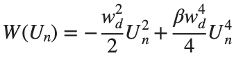
to which every coupled unit  adheres. In Eq. (1), the variable $
 $ is the unknown displacement of the oscillator occupying the n-th position of the lattice, and
  is the discretization parameter. We denote by h the distance between the oscillators of the lattice. The chain (DKG) contains linear damping with a damping coefficient
  , while
 is the coefficient of the nonlinear cubic term.
$ is the unknown displacement of the oscillator occupying the n-th position of the lattice, and For the DKG chain (1), we will consider the problem of initial-boundary values, with initial conditions

and Dirichlet boundary conditions at the boundary points  and
and  , that is,
and , that is,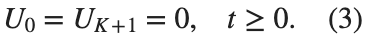
Therefore, when necessary, we will use the short notation  for the one-dimensional discrete Laplacian
for the one-dimensional discrete Laplacian
Now we want to investigate numerically the dynamics of the system (1)-(2)-(3). Our first aim is to conduct a numerical study of the property of Dynamic Stability of the system, which directly depends on the existence and linear stability of the branches of equilibrium points.
For the discussion of numerical results, it is also important to emphasize the role of the parameter  . By changing the time variable
  , we rewrite Eq. (1) in the form
 . We consider spatially extended initial conditions of the form:
We also assume zero initial velocity:
the following graphs for  and
and 
% Parameters
L = 200; % Length of the system
K = 99; % Number of spatial points
j = 2; % Mode number
omega_d = 1; % Characteristic frequency
beta = 1; % Nonlinearity parameter
delta = 0.05; % Damping coefficient
% Spatial grid
h = L / (K + 1);
n = linspace(-L/2, L/2, K+2); % Spatial points
N = length(n);
omegaDScaled = h * omega_d;
deltaScaled = h * delta;
% Time parameters
dt = 1; % Time step
tmax = 3000; % Maximum time
tspan = 0:dt:tmax; % Time vector
% Values of amplitude 'a' to iterate over
a_values = [2, 1.95, 1.9, 1.85, 1.82]; % Modify this array as needed
% Differential equation solver function
function dYdt = odefun(~, Y, N, h, omegaDScaled, deltaScaled, beta)
U = Y(1:N);
Udot = Y(N+1:end);
Uddot = zeros(size(U));
% Laplacian (discrete second derivative)
for k = 2:N-1
Uddot(k) = (U(k+1) - 2 * U(k) + U(k-1)) ;
end
% System of equations
dUdt = Udot;
dUdotdt = Uddot - deltaScaled * Udot + omegaDScaled^2 * (U - beta * U.^3);
% Pack derivatives
dYdt = [dUdt; dUdotdt];
end
% Create a figure for subplots
figure;
% Initial plot
a_init = 2; % Example initial amplitude for the initial condition plot
U0_init = a_init * sin((j * pi * h * n) / L); % Initial displacement
U0_init(1) = 0; % Boundary condition at n = 0
U0_init(end) = 0; % Boundary condition at n = K+1
subplot(3, 2, 1);
plot(n, U0_init, 'r.-', 'LineWidth', 1.5, 'MarkerSize', 10); % Line and marker plot
xlabel('$x_n$', 'Interpreter', 'latex');
ylabel('$U_n$', 'Interpreter', 'latex');
title('$t=0$', 'Interpreter', 'latex');
set(gca, 'FontSize', 12, 'FontName', 'Times');
xlim([-L/2 L/2]);
ylim([-3 3]);
grid on;
% Loop through each value of 'a' and generate the plot
for i = 1:length(a_values)
a = a_values(i);
% Initial conditions
U0 = a * sin((j * pi * h * n) / L); % Initial displacement
U0(1) = 0; % Boundary condition at n = 0
U0(end) = 0; % Boundary condition at n = K+1
Udot0 = zeros(size(U0)); % Initial velocity
% Pack initial conditions
Y0 = [U0, Udot0];
% Solve ODE
opts = odeset('RelTol', 1e-5, 'AbsTol', 1e-6);
[t, Y] = ode45(@(t, Y) odefun(t, Y, N, h, omegaDScaled, deltaScaled, beta), tspan, Y0, opts);
% Extract solutions
U = Y(:, 1:N);
Udot = Y(:, N+1:end);
% Plot final displacement profile
subplot(3, 2, i+1);
plot(n, U(end,:), 'b.-', 'LineWidth', 1.5, 'MarkerSize', 10); % Line and marker plot
xlabel('$x_n$', 'Interpreter', 'latex');
ylabel('$U_n$', 'Interpreter', 'latex');
title(['$t=3000$, $a=', num2str(a), '$'], 'Interpreter', 'latex');
set(gca, 'FontSize', 12, 'FontName', 'Times');
xlim([-L/2 L/2]);
ylim([-2 2]);
grid on;
end
% Adjust layout
set(gcf, 'Position', [100, 100, 1200, 900]); % Adjust figure size as needed
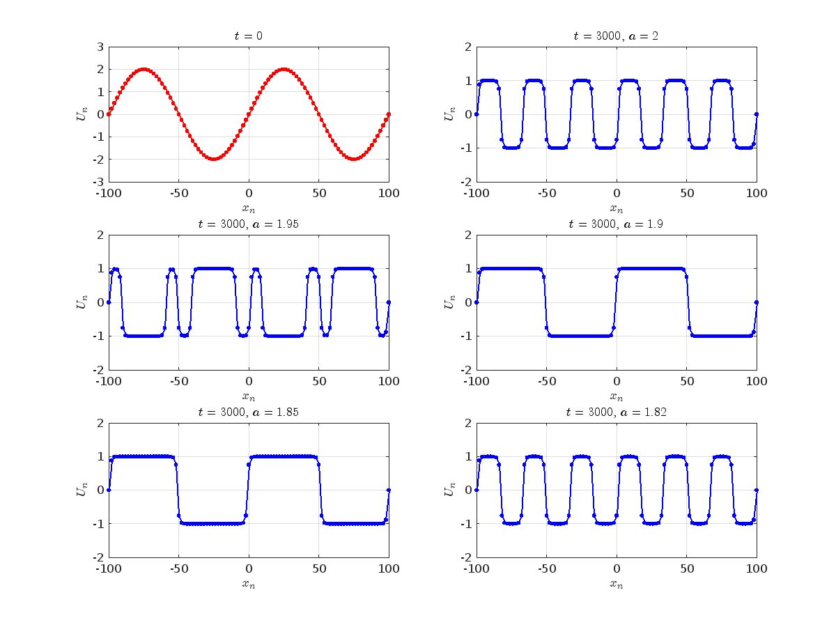
Dynamics for the initial condition ,  , for
, for  , for different amplitude values. By reducing the amplitude values, we observe the convergence to equilibrium points of different branches from
  and the appearance of values
  for which the solution converges to a non-linear equilibrium point
  Parameters:
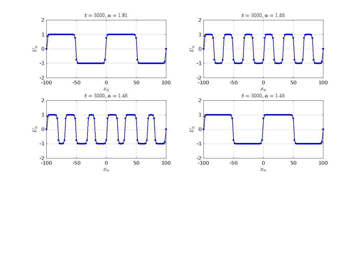
Detection of a stability threshold  : For
: For  , the initial condition ,
  , converges to a non-linear equilibrium point
 .
.
Characteristics for  , with corresponding norm
  where the dynamics appear in the first image of the third row, we observe convergence to a non-linear equilibrium point of branch
  This has the same norm and the same energy as the previous case but the final state has a completely different profile. This result suggests secondary bifurcations have occurred in branch
where the dynamics appear in the first image of the third row, we observe convergence to a non-linear equilibrium point of branch By further reducing the amplitude, distinct values of  are discerned: 1.9, 1.85, 1.81 for which the initial condition
  with norms
  respectively, converges to a non-linear equilibrium point of branch
  This equilibrium point has norm
  and energy
  . The behavior of this equilibrium is illustrated in the third row and in the first image of the third row of Figure 1, and also in the first image of the third row of Figure 2. For all the values between the aforementioned a, the initial condition
  converges to geometrically different non-linear states of branch
  as shown in the second image of the first row and the first image of the second row of Figure 2, for amplitudes
  and
and  respectively.
respectively, converges to a non-linear equilibrium point of branch and energy Refference:
There are a host of problems on Cody that require manipulation of the digits of a number. Examples include summing the digits of a number, separating the number into its powers, and adding very large numbers together.
If you haven't come across this trick yet, you might want to write it down (or save it electronically):
digits = num2str(4207) - '0'
That code results in the following:
digits =
4 2 0 7
Now, summing the digits of the number is easy:
sum(digits)
ans =
13
Hello and a warm welcome to everyone! We're excited to have you in the Cody Discussion Channel. To ensure the best possible experience for everyone, it's important to understand the types of content that are most suitable for this channel.
Content that belongs in the Cody Discussion Channel:
- Tips & tricks: Discuss strategies for solving Cody problems that you've found effective.
- Ideas or suggestions for improvement: Have thoughts on how to make Cody better? We'd love to hear them.
- Issues: Encountering difficulties or bugs with Cody? Let us know so we can address them.
- Requests for guidance: Stuck on a Cody problem? Ask for advice or hints, but make sure to show your efforts in attempting to solve the problem first.
- General discussions: Anything else related to Cody that doesn't fit into the above categories.
Content that does not belong in the Cody Discussion Channel:
- Comments on specific Cody problems: Examples include unclear problem descriptions or incorrect testing suites.
- Comments on specific Cody solutions: For example, you find a solution creative or helpful.
Please direct such comments to the Comments section on the problem or solution page itself.
We hope the Cody discussion channel becomes a vibrant space for sharing expertise, learning new skills, and connecting with others.
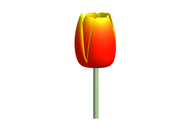
Spring is here in Natick and the tulips are blooming! While tulips appear only briefly here in Massachusetts, they provide a lot of bright and diverse colors and shapes. To celebrate this cheerful flower, here's some code to create your own tulip!
Check out this episode about PIVLab: https://www.buzzsprout.com/2107763/15106425
Join the conversation with William Thielicke, the developer of PIVlab, as he shares insights into the world of particle image velocimetery (PIV) and its applications. Discover how PIV accurately measures fluid velocities, non invasively revolutionising research across the industries. Delve into the development journey of PI lab, including collaborations, key features and future advancements for aerodynamic studies, explore the advanced hardware setups camera technologies, and educational prospects offered by PIVlab, for enhanced fluid velocity measurements. If you are interested in the hardware he speaks of check out the company: Optolution.
Let's talk about probability theory in Matlab.
Conditions of the problem - how many more letters do I need to write to the sales department to get an answer?
To get closer to the problem, I need to buy a license under a contract. Maybe sometimes there are responsible employees sitting here who will give me an answer.
Thank you
In the MATLAB description of the algorithm for Lyapunov exponents, I believe there is ambiguity and misuse.
The lambda(i) in the reference literature signifies the Lyapunov exponent of the entire phase space data after expanding by i time steps, but in the calculation formula provided in the MATLAB help documentation, Y_(i+K) represents the data point at the i-th point in the reconstructed data Y after K steps, and this calculation formula also does not match the calculation code given by MATLAB. I believe there should be some misguidance and misunderstanding here.
According to the symbol regulations in the algorithm description and the MATLAB code, I think the correct formula might be y(i) = 1/dt * 1/N * sum_j( log( ||Y_(j+i) - Y_(j*+i)|| ) )
Drumlin Farm has welcomed MATLAMB, named in honor of MathWorks, among ten adorable new lambs this season!
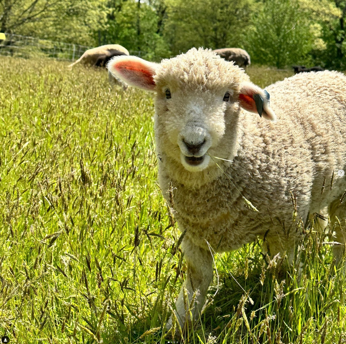
Are you local to Boston?
Shape the Future of MATLAB: Join MathWorks' UX Night In-Person!
When: June 25th, 6 to 8 PM
Where: MathWorks Campus in Natick, MA
🌟 Calling All MATLAB Users! Here's your unique chance to influence the next wave of innovations in MATLAB and engineering software. MathWorks invites you to participate in our special after-hours usability studies. Dive deep into the latest MATLAB features, share your valuable feedback, and help us refine our solutions to better meet your needs.
🚀 This Opportunity Is Not to Be Missed:
- Exclusive Hands-On Experience: Be among the first to explore new MATLAB features and capabilities.
- Voice Your Expertise: Share your insights and suggestions directly with MathWorks developers.
- Learn, Discover, and Grow: Expand your MATLAB knowledge and skills through firsthand experience with unreleased features.
- Network Over Dinner: Enjoy a complimentary dinner with fellow MATLAB enthusiasts and the MathWorks team. It's a perfect opportunity to connect, share experiences, and network after work.
- Earn Rewards: Participants will not only contribute to the advancement of MATLAB but will also be compensated for their time. Plus, enjoy special MathWorks swag as a token of our appreciation!
👉 Reserve Your Spot Now: Space is limited for these after-hours sessions. If you're passionate about MATLAB and eager to contribute to its development, we'd love to hear from you.

I found this plot of words said by different characters on the US version of The Office sitcom. There's a sparkline for each character from pilot to finale episode.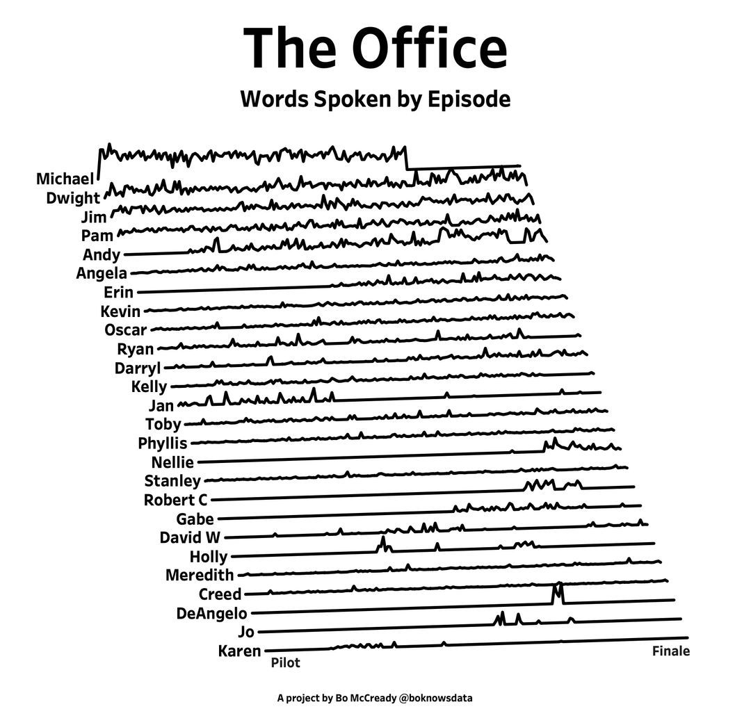
Are you a Simulink user eager to learn how to create apps with App Designer? Or an App Designer enthusiast looking to dive into Simulink?
Don't miss today's article on the Graphics and App Building Blog by @Robert Philbrick! Discover how to build Simulink Apps with App Designer, streamlining control of your simulations!
您也可以从以下列表中选择网站:
美洲
- América Latina (Español)
- Canada (English)
- United States (English)
欧洲
- Belgium (English)
- Denmark (English)
- Deutschland (Deutsch)
- España (Español)
- Finland (English)
- France (Français)
- Ireland (English)
- Italia (Italiano)
- Luxembourg (English)
- Netherlands (English)
- Norway (English)
- Österreich (Deutsch)
- Portugal (English)
- Sweden (English)
- Switzerland
- United Kingdom(English)
亚太
- Australia (English)
- India (English)
- New Zealand (English)
- 中国
- 日本Japanese (日本語)
- 한국Korean (한국어)