搜索
A colleague said that you can search the Help Center using the phrase 'Introduced in' followed by a release version. Such as, 'Introduced in R2022a'. Doing this yeilds search results specific for that release.
Seems pretty handy so I thought I'd share.
Bringing the beauty of MathWorks Natick's tulips to life through code!
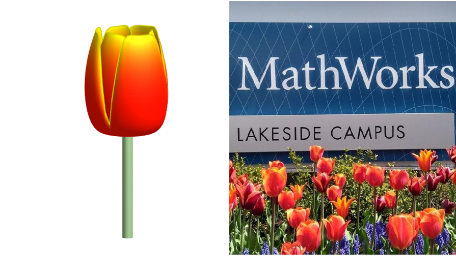
Remix challenge: create and share with us your new breeds of MATLAB tulips!
Hello MATLAB community,
I am doing some image processing with MATLAB and some issues with my coding. I just like to warn you that I am very new at coding and MATLAB so I apologise in advance for my low level and I would be very glad to have some help as I have hitted a wall, and can't find a solution to my problem.
Context: I have a video of beams, that move right to left over time. The base is fixed, only the beam moves. I converted the video to images, and my MATLAB program is going through the image file and treating every image in it. Here are two image examples:
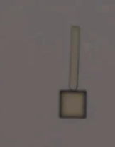 and
and 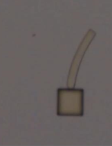
I want to measure the following things:
a. The coordinates between the 2 extremities of the beam (length of the beam, without its base), let's call them A and B.
b. The bending deformation E (L0-Lt/L0 *100), obtained by calculating the distance between A and B, called Lt.
c. the curvature of the beam (1/R), obtained by extracting the radius R of a circle fitting the curvature of the beam.
d. The angle between a vertical line passing through A, and the line AB.
What I have done so far:
My approach has been to transform my image into an rgbimage, then binaryImage, then have the complementary image, apply some modifications/corrections to the image, and then skeletonize it. And from then, I extract the coordinates of A and B, the distance between A&B (Lt), the radius of the beam R, and the angle between A&B (T).
My main issue is the skeletonisation. Because my beam is quite thick, it shortens up too much my beam, and in an inconcistent manner. So then my results are completly wrong. Here is an image of the different images and operation I have done and the result:
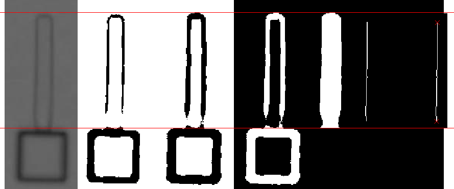
So as you can see, the length is shorter. I would like to have a skeleton that meets the edges of the beam to calculate the end points.
I have tried "bwskel(BW, 'MinBranchLength', 30)" and "bwmorph(BW, 'thin', inf)", and this: https://uk.mathworks.com/matlabcentral/fileexchange/11123-better-skeletonization. But the problem remains the same. I have tried regionpropos, but the major axis they return is too long, I have tried bwferet(), but the maxlength is in diagonal of the beam... I have running out of ideas.
Problem: So I guess my main problem is how can I get a skeletonisation that goes to the edges of the beam?
Here is my code:
for i = TrackingStart:TrackingEnd
FileRGB(:,:,i) = rgb2gray(imread(IMG)); % Convert to grayscale
croppedRGB = FileRGB(y3left:y3right, x3left:x3right, i);
binaryImage = imbinarize(croppedRGB, 'adaptive', 'ForegroundPolarity','dark','Sensitivity', 0.50);
out = nnz(~binaryImage);
while out <= 4300 % Change threshold if needed
for j = 1:50
sensitivity = 0.50 + j * 0.01;
binaryImage = imbinarize(croppedRGB, 'adaptive', 'ForegroundPolarity', 'dark', 'Sensitivity', sensitivity);
out = nnz(~binaryImage);
if out >= 4325
break; % Exit the loop if the condition is met
end
end
end
% Create a line Model
BW = imcomplement(binaryImage);
BW(y1left:y1right, x1left:x1right) = 1; % there is always sample at the junction area (between beam and base)
BW(y2left:y2right, x2left:x2right) = 0; % Always = 0 if no sample here
BW = bwmorph(BW, 'close', Inf);
BW = bwmorph(BW, 'bridge');
BW = bwareafilt(BW, 1);
s = regionprops(BW, 'FilledImage');
BW = s.FilledImage;
BW = bwskel(BW, 'MinBranchLength', 30);
endpoints = bwmorph(BW, 'endpoints');
[y_end, x_end] = find(endpoints == 1);
%Degree of bending deformation method
Lt = sqrt(power(x_end(1)-x_end(2),2)+power(y_end(1)-y_end(2),2));
if x_end(2) > x_end(1)
Lt = -Lt;
end
Lstore(i) = Lt;
%Curvature method
[row_dots_cir, col_dots_cir, val] = find(BW == 1);
[xc(i),yc(i),Rstore(i),a] = circfit(col_dots_cir,row_dots_cir);
%Angle method
slope_endpoints = (x_end(1) - x_end(2)) / (y_end(1) - y_end(2));
angle_radians = atan(slope_endpoints);
angle_degrees = rad2deg(angle_radians);
if x_end(2) > x_end(1)
angle_degrees = -angle_degrees;
end
Tstore(i) = angle_degrees;
i
end
I found this plot of words said by different characters on the US version of The Office sitcom. There's a sparkline for each character from pilot to finale episode.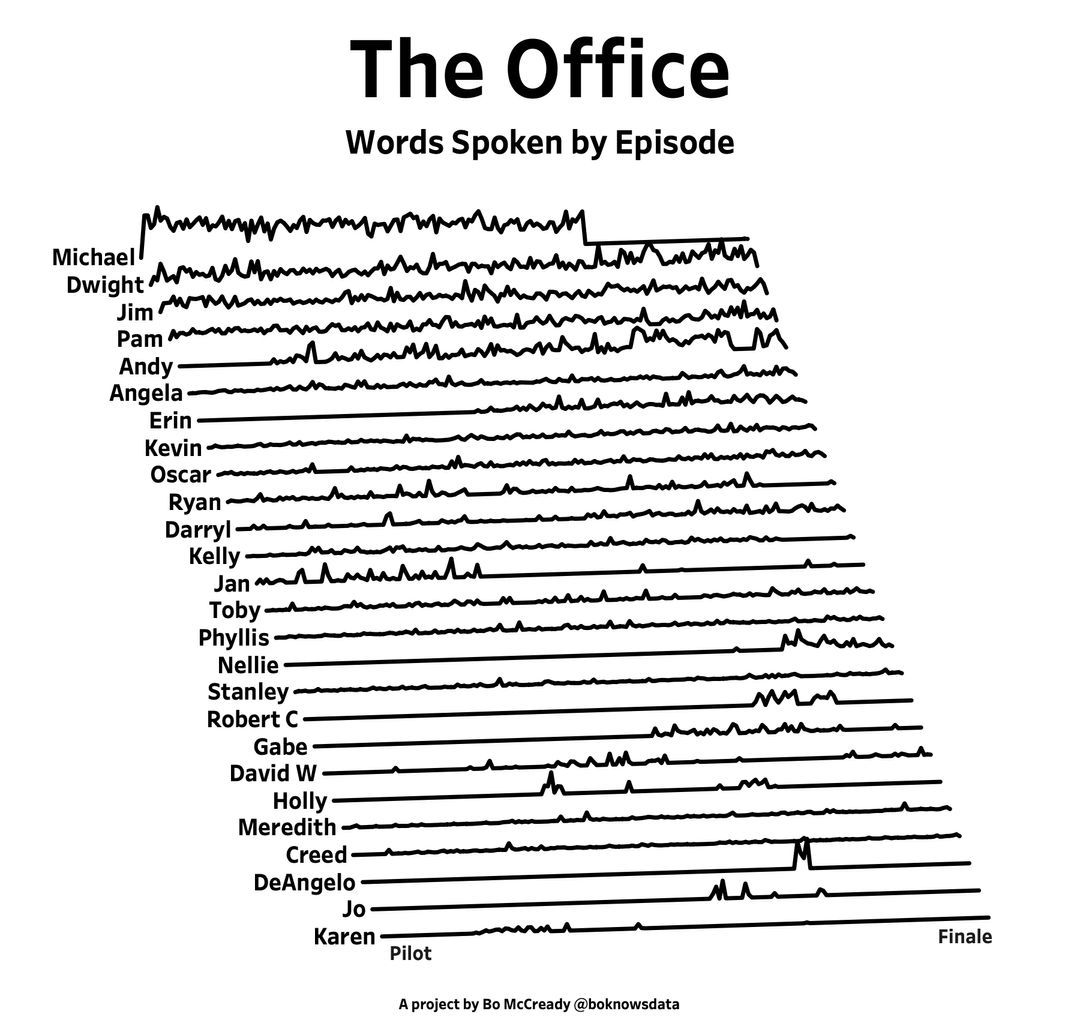
RGB triplet [0,1]
9%
RGB triplet [0,255]
12%
Hexadecimal Color Code
13%
Indexed color
16%
Truecolor array
37%
Equally unfamiliar with all-above
13%
2784 个投票
A high school student called for help with this physics problem:
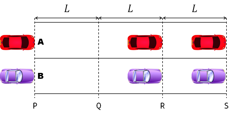
- Car A moves with constant velocity v.
- Car B starts to move when Car A passes through the point P.
- Car B undergoes...
- uniform acc. motion from P to Q.
- uniform velocity motion from Q to R.
- uniform acc. motion from R to S.
- Car A and B pass through the point R simultaneously.
- Car A and B arrive at the point S simultaneously.
Q1. When car A passes the point Q, which is moving faster?
Q2. Solve the time duration for car B to move from P to Q using L and v.
Q3. Magnitude of acc. of car B from P to Q, and from R to S: which is bigger?
Well, it can be solved with a series of tedious equations. But... how about this?
Code below:
%% get images and prepare stuffs
figure(WindowStyle="docked"),
ax1 = subplot(2,1,1);
hold on, box on
ax1.XTick = [];
ax1.YTick = [];
A = plot(0, 1, 'ro', MarkerSize=10, MarkerFaceColor='r');
B = plot(0, 0, 'bo', MarkerSize=10, MarkerFaceColor='b');
[carA, ~, alphaA] = imread('https://cdn.pixabay.com/photo/2013/07/12/11/58/car-145008_960_720.png');
[carB, ~, alphaB] = imread('https://cdn.pixabay.com/photo/2014/04/03/10/54/car-311712_960_720.png');
carA = imrotate(imresize(carA, 0.1), -90);
carB = imrotate(imresize(carB, 0.1), 180);
alphaA = imrotate(imresize(alphaA, 0.1), -90);
alphaB = imrotate(imresize(alphaB, 0.1), 180);
carA = imagesc(carA, AlphaData=alphaA, XData=[-0.1, 0.1], YData=[0.9, 1.1]);
carB = imagesc(carB, AlphaData=alphaB, XData=[-0.1, 0.1], YData=[-0.1, 0.1]);
txtA = text(0, 0.85, 'A', FontSize=12);
txtB = text(0, 0.17, 'B', FontSize=12);
yline(1, 'r--')
yline(0, 'b--')
xline(1, 'k--')
xline(2, 'k--')
text(1, -0.2, 'Q', FontSize=20, HorizontalAlignment='center')
text(2, -0.2, 'R', FontSize=20, HorizontalAlignment='center')
% legend('A', 'B') % this make the animation slow. why?
xlim([0, 3])
ylim([-.3, 1.3])
%% axes2: plots velocity graph
ax2 = subplot(2,1,2);
box on, hold on
xlabel('t'), ylabel('v')
vA = plot(0, 1, 'r.-');
vB = plot(0, 0, 'b.-');
xline(1, 'k--')
xline(2, 'k--')
xlim([0, 3])
ylim([-.3, 1.8])
p1 = patch([0, 0, 0, 0], [0, 1, 1, 0], [248, 209, 188]/255, ...
EdgeColor = 'none', ...
FaceAlpha = 0.3);
%% solution
v = 1; % car A moves with constant speed.
L = 1; % distances of P-Q, Q-R, R-S
% acc. of car B for three intervals
a(1) = 9*v^2/8/L;
a(2) = 0;
a(3) = -1;
t_BatQ = sqrt(2*L/a(1)); % time when car B arrives at Q
v_B2 = a(1) * t_BatQ; % speed of car B between Q-R
%% patches for velocity graph
p2 = patch([t_BatQ, t_BatQ, t_BatQ, t_BatQ], [1, 1, v_B2, v_B2], ...
[248, 209, 188]/255, ...
EdgeColor = 'none', ...
FaceAlpha = 0.3);
p3 = patch([2, 2, 2, 2], [1, v_B2, v_B2, 1], [194, 234, 179]/255, ...
EdgeColor = 'none', ...
FaceAlpha = 0.3);
%% animation
tt = linspace(0, 3, 2000);
for t = tt
A.XData = v * t;
vA.XData = [vA.XData, t];
vA.YData = [vA.YData, 1];
if t < t_BatQ
B.XData = 1/2 * a(1) * t^2;
vB.XData = [vB.XData, t];
vB.YData = [vB.YData, a(1) * t];
p1.XData = [0, t, t, 0];
p1.YData = [0, vB.YData(end), 1, 1];
elseif t >= t_BatQ && t < 2
B.XData = L + (t - t_BatQ) * v_B2;
vB.XData = [vB.XData, t];
vB.YData = [vB.YData, v_B2];
p2.XData = [t_BatQ, t, t, t_BatQ];
p2.YData = [1, 1, vB.YData(end), vB.YData(end)];
else
B.XData = 2*L + v_B2 * (t - 2) + 1/2 * a(3) * (t-2)^2;
vB.XData = [vB.XData, t];
vB.YData = [vB.YData, v_B2 + a(3) * (t - 2)];
p3.XData = [2, t, t, 2];
p3.YData = [1, 1, vB.YData(end), v_B2];
end
txtA.Position(1) = A.XData(end);
txtB.Position(1) = B.XData(end);
carA.XData = A.XData(end) + [-.1, .1];
carB.XData = B.XData(end) + [-.1, .1];
drawnow
end
I have question about using 'bnlssm' object when the problem involves time-varying coefs. Per this documentation https://www.mathworks.com/help/econ/bnlssm.html , bnlssm allows the transition matrix to be a nonlinear function of the past values of the state vector, while also being time-varying --, i.e. A_t(x_{t-1}). However the documentation contains an example of the parameter mapping function for a fixed coef. case only:
function [A,B,C,D,Mean0,Cov0,StateType] = paramMap(theta)
A = @(x)blkdiag([theta(1) theta(2); 0 1],[theta(3) theta(4); 0 1])*x;
B = [theta(5) 0; 0 0; 0 theta(6); 0 0];
C = @(x)log(exp(x(1)-theta(2)/(1-theta(1))) + ...
exp(x(3)-theta(4)/(1-theta(3))));
D = theta(7);
Mean0 = [theta(2)/(1-theta(1)); 1; theta(4)/(1-theta(3)); 1];
Cov0 = diag([theta(5)^2/(1-theta(1)^2) 0 theta(6)^2/(1-theta(3)^2) 0]);
StateType = [0; 1; 0; 1]; % Stationary state and constant 1 processes
end
Here, A and C are recognised as function handles and show the dimension of 1-by-1 when [A,B,C,D]=paramMap(theta) is run with a given theta. This does not prevent filter/smooth from returning the states estimates, as the function handles become m-by-m matices when the function handles are evaluated.
However, whenever I try replaceing A with a cell array, e.g.:
A=cell(T,1);
for t=1:T
A{t} = @(x)blkdiag([theta(1) theta(2); 0 1],[theta(3) theta(4); 0 1])*x;
end
bnlssm.fixcoeff throws an error that the dimensions of Mean0 are expected to be 1, per validation step in lines 700-707 of 'bnlssm.m':
if iscellA; At = A{1};
else; At = A; end
numStates0 = size(At,2);
if
isscalar(mean0)
mean0 = mean0(ones(numStates0,1),:);
elseif
~isempty(mean0)
mean0 = mean0(:);
validateattributes(mean0,{'numeric'},{'finite','real','numel',numStates0},callerName,'Mean0');
end
Q: Is it just overlook by MathWorks programmers and creating local verions of bnlssm/filter/smooth with that validation step removed is a viable pathway forward, or is it intentional because 'bnlssm' was in fact designed to handle only the time-invariant coef. case correctly?
is there any sites available online free ai course learning except: coursera.org
From Alpha Vantage's website: API Documentation | Alpha Vantage
Try using the built-in Matlab function webread(URL)... for example:
% copy a URL from the examples on the site
URL = 'https://www.alphavantage.co/query?function=TIME_SERIES_DAILY&symbol=IBM&apikey=demo'
% or use the pattern to create one
tickers = [{'IBM'} {'SPY'} {'DJI'} {'QQQ'}]; i = 1;
URL = ...
['https://www.alphavantage.co/query?function=TIME_SERIES_DAILY_ADJUSTED&outputsize=full&symbol=', ...
+ tickers{i}, ...
+ '&apikey=***Put Your API Key here***'];
X = webread(URL);
You can access any of the data available on the site as per the Alpha Vantage documentation using these two lines of code but with different designations for the requested data as per the documentation.
It's fun!
isstring
11%
ischar
7%
iscellstr
13%
isletter
21%
isspace
9%
ispunctuation
37%
2455 个投票
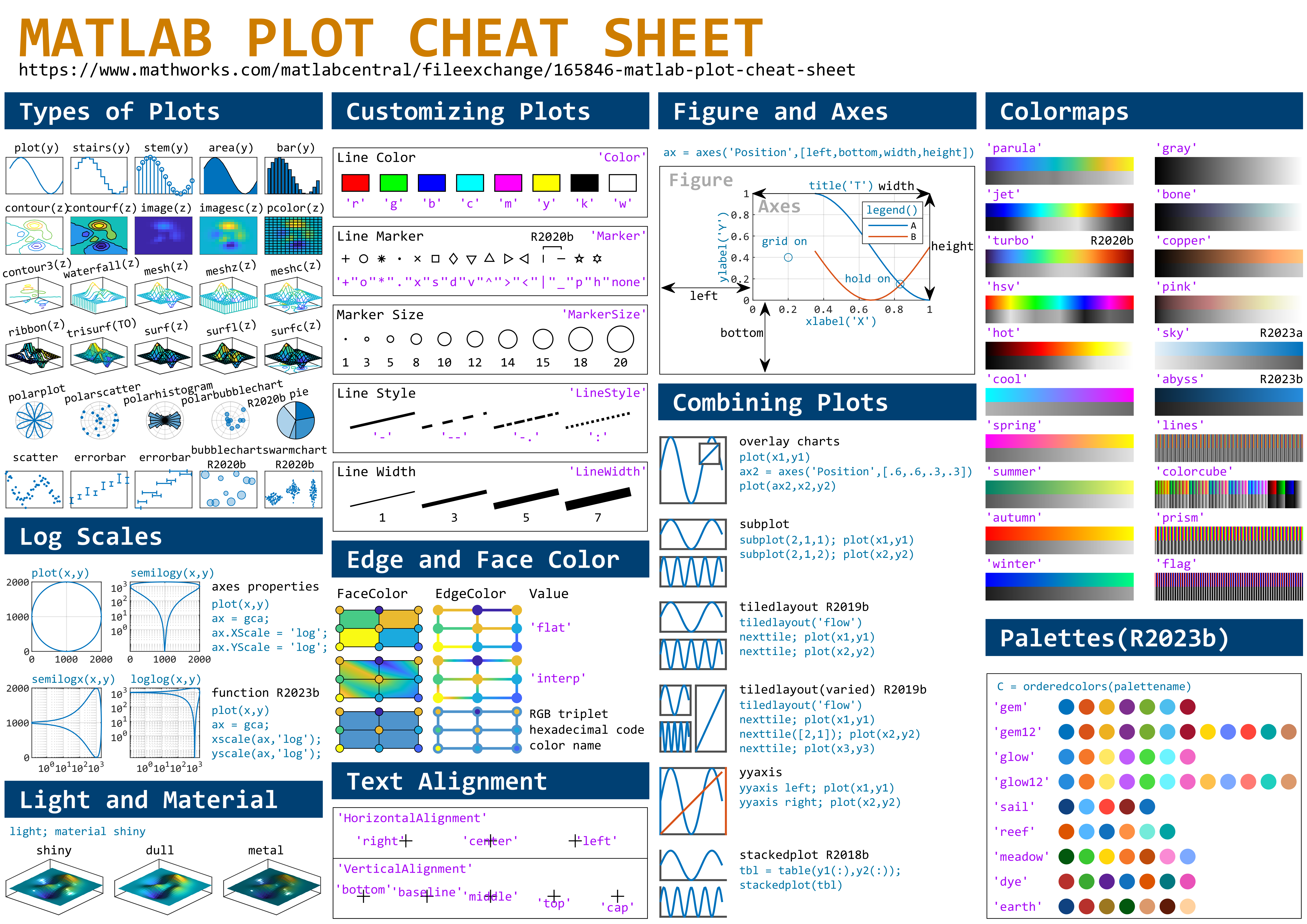
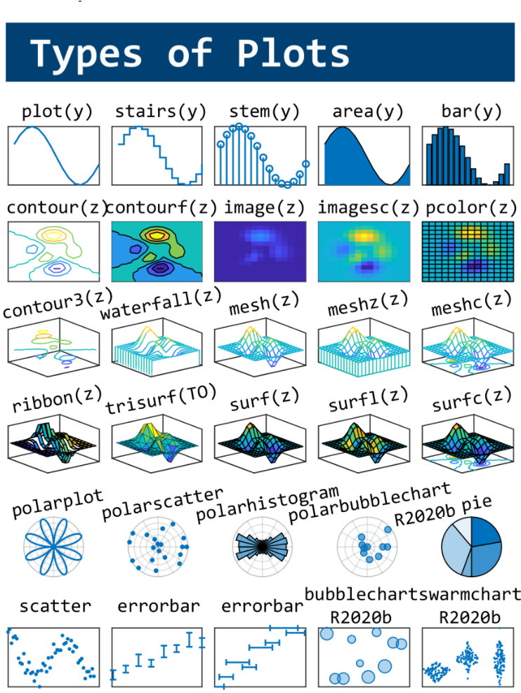
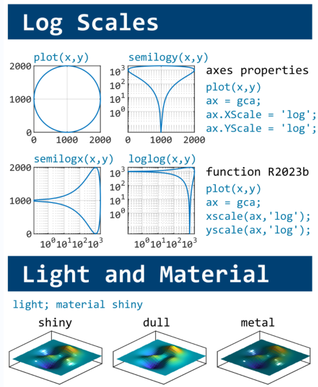
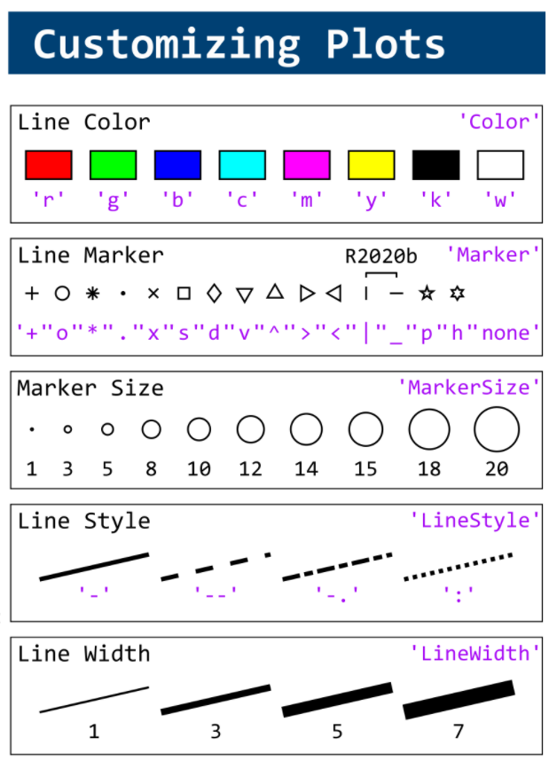
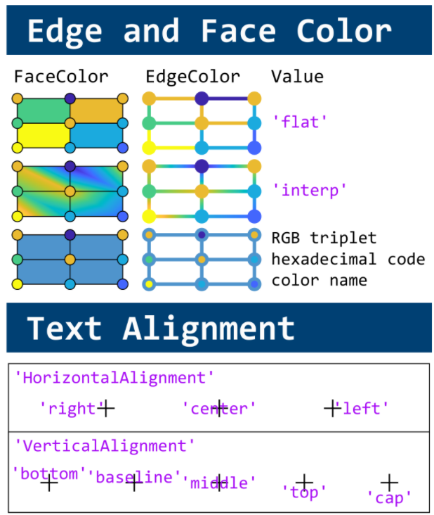
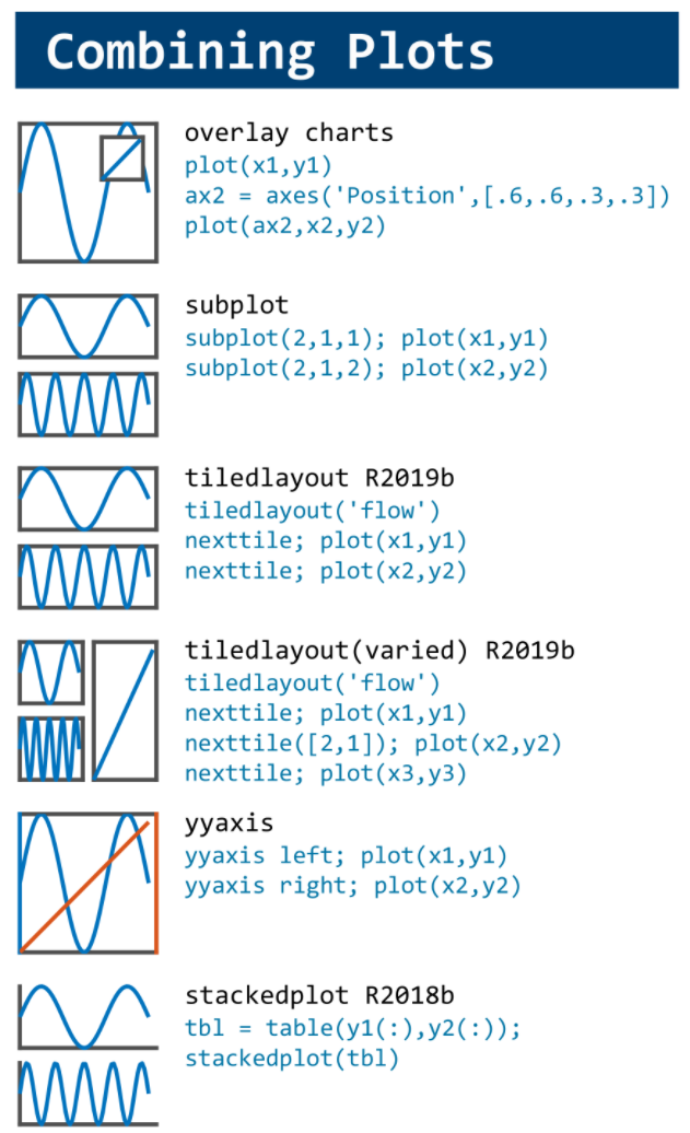
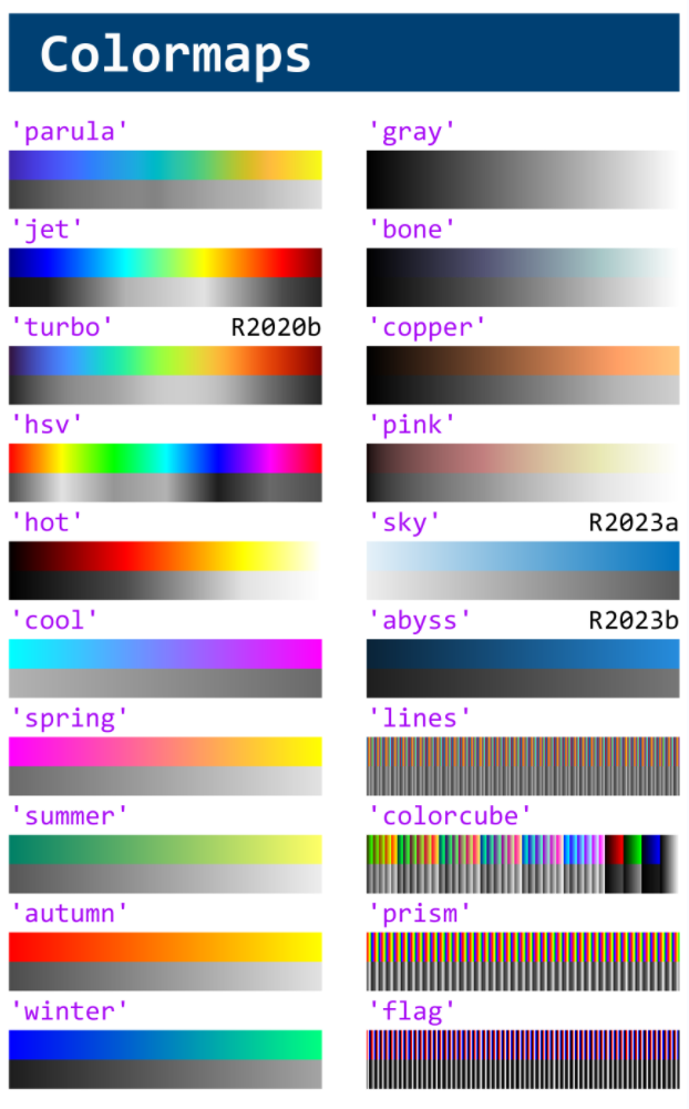
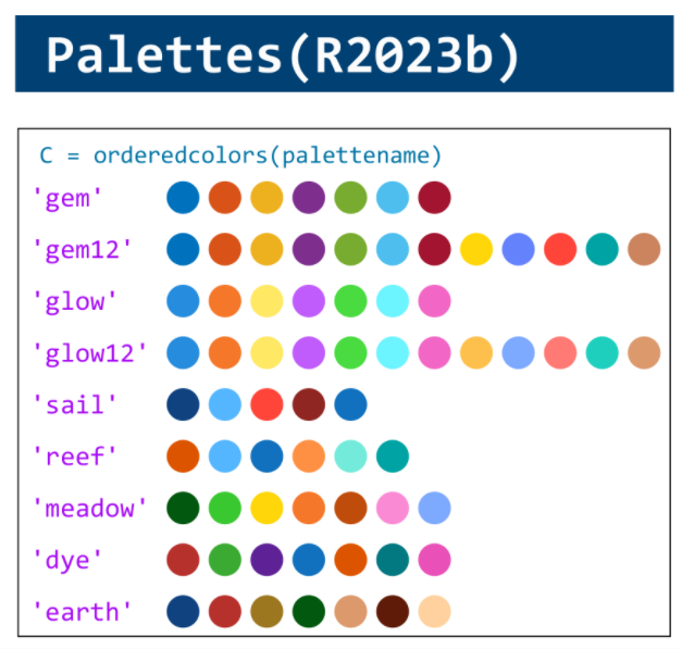
This cheat sheet is here:
reference:
- https://github.com/peijin94/matlabPlotCheatsheet
- https://github.com/mathworks/visualization-cheat-sheet
- https://www.mathworks.com/products/matlab/plot-gallery.html
- https://www.mathworks.com/help/matlab/release-notes.html
MATLAB used to have official visualization-cheat-sheet, but there have been quite a few new updates in MATLAB versions recently. Therefore, I made my own cheat sheet and marked the versions of each new thing that were released :
If structure is in the form of struct1.struct2(m,n).struct3. how to extract values present in struct3 using mex function
Dear MATLAB contest enthusiasts,
I believe many of you have been captivated by the innovative entries from Zhaoxu Liu / slanderer, in the 2023 MATLAB Flipbook Mini Hack contest.


Ever wondered about the person behind these creative entries? What drives a MATLAB user to such levels of skill? And what inspired his participation in the contest? We were just as curious as you are!
We were delighted to catch up with him and learn more about his use of MATLAB. The interview has recently been published in MathWorks Blogs. For an in-depth look into his insights and experiences, be sure to read our latest blog post: Community Q&A – Zhaoxu Liu.
But the conversation doesn't end here! Who would you like to see featured in our next interview? Drop their name in the comments section below and let us know who we should reach out to next!
Hey MATLAB Community! 🌟
In the vibrant landscape of our online community, the past few weeks have been particularly exciting. We've seen a plethora of contributions that not only enrich our collective knowledge but also foster a spirit of collaboration and innovation. Here are some of the noteworthy contributions from our members.
Interesting Questions
Victor encountered a puzzling error while trying to publish his script to PDF. His post sparked a helpful discussion on troubleshooting this issue, proving invaluable for anyone facing similar challenges.
Devendra's inquiry into interpolating and smoothing NDVI time series using MATLAB has opened up a dialogue on various techniques to manage noisy data, benefiting researchers and enthusiasts in the field of remote sensing.
Popular Discussions
Adam Danz's AMA session has been a treasure trove of insights into the workings behind the MATLAB Answers forum, offering a unique perspective from a staff contributor's viewpoint.
The User Following feature marks a significant enhancement in how community members can stay connected with the contributions of their peers, fostering a more interconnected MATLAB Central.
From File Exchange
Robert Haaring's submission is a standout contribution, providing a sophisticated model for CO2 electrolysis, a topic of great relevance to researchers in environmental technology and chemical engineering.
From the Blogs
Verification and Validation for AI: From model implementation to requirements validation by Sivylla Paraskevopoulou
Sivylla's comprehensive post delves into the critical stages of AI model development, from implementation to validation, offering invaluable guidance for professionals navigating the complexities of AI verification.
In this engaging Q&A, Ned Gulley introduces us to Zhaoxu Liu, a remarkable community member whose innovative contributions and active engagement have left a significant impact on the MATLAB community.
Each of these contributions highlights the diverse and rich expertise within our community. From solving complex technical issues to introducing new features and sharing in-depth knowledge on specialized topics, our members continue to make MATLAB Central a vibrant and invaluable resource.
Let's continue to support, inspire, and learn from one another
Don't use / What are Projects?
26%
1–10
31%
11–20
15%
21–30
9%
31–50
7%
51+ (comment below)
12%
4070 个投票
Updating some of my educational Livescripts to 2024a, really love the new "define a function anywhere" feature, and have a "new" idea for improving Livescripts -- support "hidden" code blocks similar to the Jupyter Notebooks functionality.
For example, I often create "complicated" plots with a bunch of ancillary items and I don't want this code exposed to the reader by default, as it might confuse the reader. For example, consider a Livescript that might read like this:
-----
Noting the similar structure of these two mappings, let's now write a function that simply maps from some domain to some other domain using change of variable.
function x = ChangeOfVariable( x, from_domain, to_domain )
x = x - from_domain(1);
x = x * ( ( to_domain(2) - to_domain(1) ) / ( from_domain(2) - from_domain(1) ) );
x = x + to_domain(1);
end
Let's see this function in action
% HIDE CELL
clear
close all
from_domain = [-1, 1];
to_domain = [2, 7];
from_values = [-1, -0.5, 0, 0.5, 1];
to_values = ChangeOfVariable( from_values, from_domain, to_domain )
to_values = 1×5
2.0000 3.2500 4.5000 5.7500 7.0000
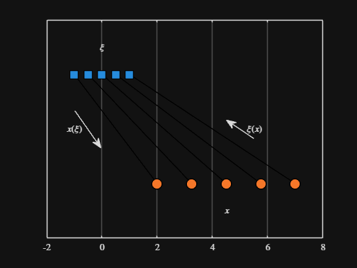
We can plot the values of from_values and to_values, showing how they're connected to each other:
% HIDE CELL
figure
hold on
for n = 1 : 5
plot( [from_values(n) to_values(n)], [1 0], Color="k", LineWidth=1 )
end
ax = gca;
ax.YTick = [];
ax.XLim = [ min( [from_domain, to_domain] ) - 1, max( [from_domain, to_domain] ) + 1 ];
ax.YLim = [-0.5, 1.5];
ax.XGrid = "on";
scatter( from_values, ones( 5, 1 ), Marker="s", MarkerFaceColor="flat", MarkerEdgeColor="k", SizeData=120, LineWidth=1, SeriesIndex=1 )
text( mean( from_domain ), 1.25, "$\xi$", Interpreter="latex", HorizontalAlignment="center", VerticalAlignment="middle" )
scatter( to_values, zeros( 5, 1 ), Marker="o", MarkerFaceColor="flat", MarkerEdgeColor="k", SizeData=120, LineWidth=1, SeriesIndex=2 )
text( mean( to_domain ), -0.25, "$x$", Interpreter="latex", HorizontalAlignment="center", VerticalAlignment="middle" )
scaled_arrow( ax, [mean( [from_domain(1), to_domain(1) ] ) - 1, 0.5], ( 1 - 0 ) / ( from_domain(1) - to_domain(1) ), 1 )
scaled_arrow( ax, [mean( [from_domain(end), to_domain(end)] ) + 1, 0.5], ( 1 - 0 ) / ( from_domain(end) - to_domain(end) ), -1 )
text( mean( [from_domain(1), to_domain(1) ] ) - 1.5, 0.5, "$x(\xi)$", Interpreter="latex", HorizontalAlignment="center", VerticalAlignment="middle" )
text( mean( [from_domain(end), to_domain(end)] ) + 1.5, 0.5, "$\xi(x)$", Interpreter="latex", HorizontalAlignment="center", VerticalAlignment="middle" )
-----
Where scaled_arrow is some utility function I've defined elsewhere... See how a majority of the code is simply "drivel" to create the plot, clear and close? I'd like to be able to hide those cells so that it would look more like this:
-----
Noting the similar structure of these two mappings, let's now write a function that simply maps from some domain to some other domain using change of variable.
function x = ChangeOfVariable( x, from_domain, to_domain )
x = x - from_domain(1);
x = x * ( ( to_domain(2) - to_domain(1) ) / ( from_domain(2) - from_domain(1) ) );
x = x + to_domain(1);
end
Let's see this function in action
▶ Show code cell
from_domain = [-1, 1];
to_domain = [2, 7];
from_values = [-1, -0.5, 0, 0.5, 1];
to_values = ChangeOfVariable( from_values, from_domain, to_domain )
to_values = 1×5
2.0000 3.2500 4.5000 5.7500 7.0000
We can plot the values of from_values and to_values, showing how they're connected to each other:
▶ Show code cell

-----
Thoughts?
I recently had issues with code folding seeming to disappear and it turns out that I had unknowingly disabled the "show code folding margin" option by accident. Despite using MATLAB for several years, I had no idea this was an option, especially since there seemed to be no references to it in the code folding part of the "Preferences" menu.
It would be great if in the future, there was a warning that told you about this when you try enable/disable folding in the Preferences.
I am using 2023b by the way.
i want to communicate matlab simulink and F28379D launchpad. initally i want to blink LED of launchpad by using serial communication, i didnt understand hoiw can i do that?
I have attached its figure of my matlab simulink model with it. can anyone guide me?
2
17%
3
12%
4
59%
6
4%
8
5%
Other (comment below)
3%
6419 个投票
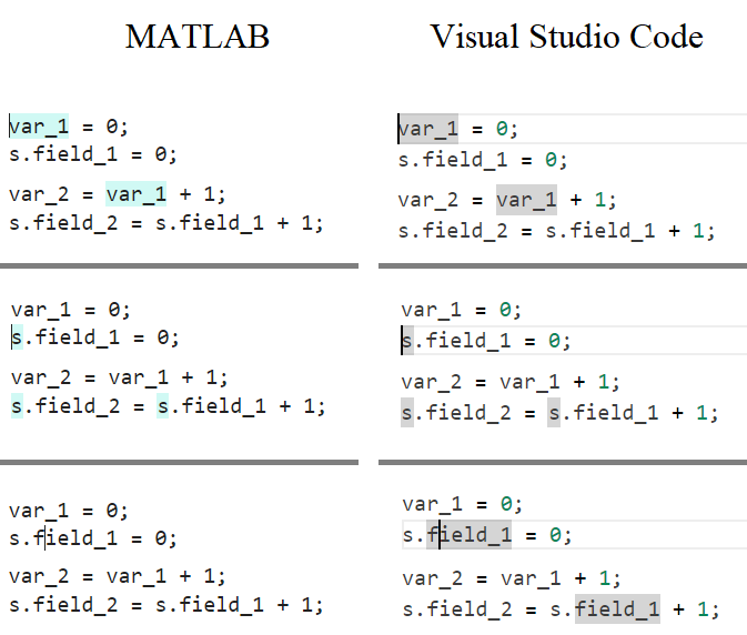
In the MATLAB editor, when clicking on a variable name, all the other instances of the variable name will be highlighted.
But this does not work for structure fields, which is a pity. Such feature would be quite often useful for me.
I show an illustration below, and compare it with Visual Studio Code that does it. ;-)
I am using MATLAB R2023a, sorry if it has been added to newer versions, but I didn't see it in the release notes.