eqn =
主要内容
搜索
I am curious as to how my goal can be accomplished in Matlab.
The present APP called "Matching Network Designer" works quite well, but it is limited to a single section of a "PI", a "TEE", or an "L" topology circuit.
This limits the bandwidth capability of the APP when the intended use is to create an amplifier design intended for wider bandwidth projects.
I am requesting that a "Broadband Matching Network Designer" APP be developed by you, the MathWorks support team.
One suggestion from me is to be able to cascade a second section (or "pole") to the first.
Then the resulting topology would be capable of achieving that wider bandwidth of the microwave amplifier project where it would be later used with the transistor output and input matching networks.
Instead of limiting the APP to a single frequency, the entire s parameter file would be used as an input.
The APP would convert the polar s parameters to rectangular scaler complex impedances that you already use.
At that point, having started out with the first initial center frequency, the other frequencies both greater than and less than the center would come into use by an optimization of the circuit elements.
I'm hoping that you will be able to take on this project.
I can include an attachment of such a Matching Network Designer APP that you presently have if you like.
That network is centered at 10 GHz.
Kimberly Renee Alvarez.
310-367-5768
Hello,
Now that the "Copilot+PC" (Windows ARM) laptops are rapidly increasing in market share (Microsoft Surface Laptop, Dell XPS 13, HP OmniBook X 14, and more), are there any plans to provide builds for Matlab on Windows arm64?
Since there are already Windows builds of Matlab, it shouldn't be too hard to compile for Windows arm64, as far as I know. But I am not famaliar with Matlab's codebase.
Please try to publish Windows arm64 builds soon so that Matlab can be much more usable on Windows on ARM as it will run natively instead of in emulation.
Thank you very much.
Attaching the Photoshop file if you want to modify the caption.
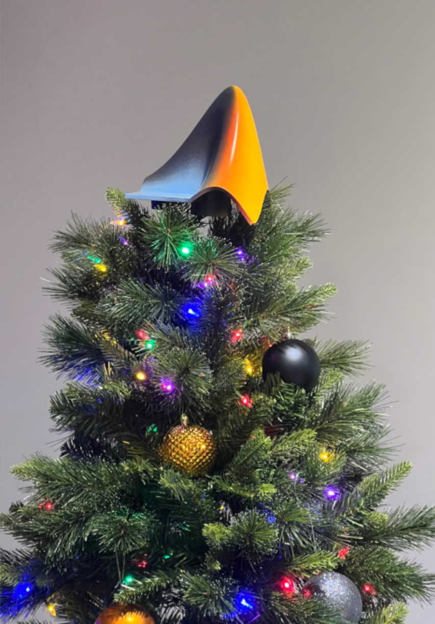
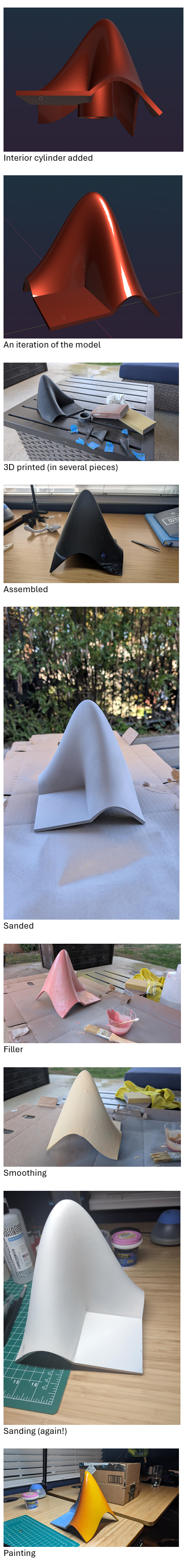
What better way to add a little holiday magic than the L-shaped membrane atop your evergreen? My colleagues output the shape and then added some thickness and an interior cylinder in Blender. Then, the shape was exported to STL and 3D printed (in several pieces). Then glued, sanded, primed, sanded again and painted. If you like, the STL file is attached. Thank you to https://blogs.mathworks.com/community/2013/06/20/paul-prints-the-l-shaped-membrane/ and a tip of the hat to MATLAB Ornament. Happy Holidays!
If you have a folder with an enormous number of files and want to use the uigetfile function to select specific files, you may have noticed a significant delay in displaying the file list.
Thanks to the assistance from MathWorks support, an interesting behavior was observed.
For example, if a folder such as Z:\Folder1\Folder2\data contains approximately 2 million files, and you attempt to use uigetfile to access files with a specific extension (e.g., *.ext), the following behavior occurs:
Method 1: This takes minutes to show me the list of all files
[FileName, PathName] = uigetfile('Z:\Folder1\Folder2\data\*.ext', 'File selection');
Method 2: This takes less than a second to display all files.
[FileName, PathName] = uigetfile('*.ext', 'File selection','Z:\Folder1\Folder2\data');
Method 3: This method also takes minutes to display the file list. What is intertesting is that this method is the same as Method 2, except that a file seperator "\" is added at the end of the folder string.
[FileName, PathName] = uigetfile('*.ext', 'File selection','Z:\Folder1\Folder2\data\');
I was informed that the Mathworks development team has been informed of this strange behaviour.
I am using 2023a, but think this should be the same for newer versions.
This post is more of a "tips and tricks" guide than a question.
If you have a folder with an enormous number of files and want to use the uigetfile function to select specific files, you may have noticed a significant delay in displaying the file list.
Thanks to the assistance from MathWorks support, an interesting behavior was observed.
For example, if a folder such as Z:\Folder1\Folder2\data contains approximately 2 million files, and you attempt to use uigetfile to access files with a specific extension (e.g., *.ext), the following behavior occurs:
Method 1: This takes minutes to show me the list of all files
[FileName, PathName] = uigetfile('Z:\Folder1\Folder2\data\*.ext', 'File selection');
Method 2: This takes less than a second to display all files.
[FileName, PathName] = uigetfile('*.ext', 'File selection','Z:\Folder1\Folder2\data');
Method 3: This method also takes minutes to display the file list. What is intertesting is that this method is the same as Method 2, except that a file seperator "\" is added at the end of the folder string.
[FileName, PathName] = uigetfile('*.ext', 'File selection','Z:\Folder1\Folder2\data\');
I was informed that the Mathworks development team has been informed of this strange behaviour.
I am using 2023a, but think this should be the same for newer versions.

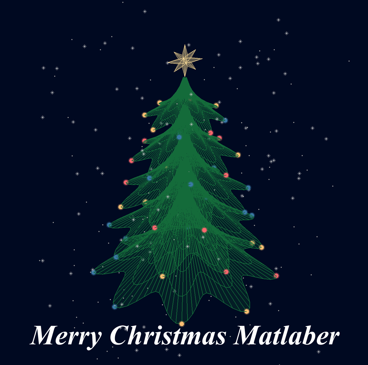
Christmas is coming, here are two dynamic Christmas tree drawing codes:
Crystal XMas Tree
function XmasTree2024_1
fig = figure('Units','normalized', 'Position',[.1,.1,.5,.8],...
'Color',[0,9,33]/255, 'UserData',40 + [60,65,75,72,0,59,64,57,74,0,63,59,57,0,1,6,45,75,61,74,28,57,76,57,1,1]);
axes('Parent',fig, 'Position',[0,-1/6,1,1+1/3], 'UserData',97 + [18,11,0,13,3,0,17,4,17],...
'XLim',[-1.5,1.5], 'YLim',[-1.5,1.5], 'ZLim',[-.2,3.8], 'DataAspectRatio', [1,1,1], 'NextPlot','add',...
'Projection','perspective', 'Color',[0,9,33]/255, 'XColor','none', 'YColor','none', 'ZColor','none')
%% Draw Christmas tree
F = [1,3,4;1,4,5;1,5,6;1,6,3;...
2,3,4;2,4,5;2,5,6;2,6,3];
dP = @(V) patch('Faces',F, 'Vertices',V, 'FaceColor',[0 71 177]./255,...
'FaceAlpha',rand(1).*0.2+0.1, 'EdgeColor',[0 71 177]./255.*0.8,...
'EdgeAlpha',0.6, 'LineWidth',0.5, 'EdgeLighting','gouraud', 'SpecularStrength',0.3);
r = .1; h = .8;
V0 = [0,0,0; 0,0,1; 0,r,h; r,0,h; 0,-r,h; -r,0,h];
% Rotation matrix
Rx = @(V, theta) V*[1 0 0; 0 cos(theta) sin(theta); 0 -sin(theta) cos(theta)];
Rz = @(V, theta) V*[cos(theta) sin(theta) 0;-sin(theta) cos(theta) 0; 0 0 1];
N = 180; Vn = zeros(N, 3); eval(char(fig.UserData))
for i = 1:N
tV = Rz(Rx(V0.*(1.2 - .8.*i./N + rand(1).*.1./i^(1/5)), pi/3.*(1 - .6.*i./N)), i.*pi/8.1 + .001.*i.^2) + [0,0,.016.*i];
dP(tV); Vn(i,:) = tV(2,:);
end
scatter3(Vn(:,1).*1.02,Vn(:,2).*1.02,Vn(:,3).*1.01, 30, 'w', 'Marker','*', 'MarkerEdgeAlpha',.5)
%% Draw Star of Bethlehem
w = .3; R = .62; r = .4; T = (1/8:1/8:(2 - 1/8)).'.*pi;
V8 = [ 0, 0, w; 0, 0,-w;
1, 0, 0; 0, 1, 0; -1, 0, 0; 0,-1,0;
R, R, 0; -R, R, 0; -R,-R, 0; R,-R,0;
cos(T).*r, sin(T).*r, T.*0];
F8 = [1,3,25; 1,3,11; 2,3,25; 2,3,11; 1,7,11; 1,7,13; 2,7,11; 2,7,13;
1,4,13; 1,4,15; 2,4,13; 2,4,15; 1,8,15; 1,8,17; 2,8,15; 2,8,17;
1,5,17; 1,5,19; 2,5,17; 2,5,19; 1,9,19; 1,9,21; 2,9,19; 2,9,21;
1,6,21; 1,6,23; 2,6,21; 2,6,23; 1,10,23; 1,10,25; 2,10,23; 2,10,25];
V8 = Rx(V8.*.3, pi/2) + [0,0,3.5];
patch('Faces',F8, 'Vertices',V8, 'FaceColor',[255,223,153]./255,...
'EdgeColor',[255,223,153]./255, 'FaceAlpha', .2)
%% Draw snow
sXYZ = rand(200,3).*[4,4,5] - [2,2,0];
sHdl1 = plot3(sXYZ(1:90,1),sXYZ(1:90,2),sXYZ(1:90,3), '*', 'Color',[.8,.8,.8]);
sHdl2 = plot3(sXYZ(91:200,1),sXYZ(91:200,2),sXYZ(91:200,3), '.', 'Color',[.6,.6,.6]);
annotation(fig,'textbox',[0,.05,1,.09], 'Color',[1 1 1], 'String','Merry Christmas Matlaber',...
'HorizontalAlignment','center', 'FontWeight','bold', 'FontSize',48,...
'FontName','Times New Roman', 'FontAngle','italic', 'FitBoxToText','off','EdgeColor','none');
% Rotate the Christmas tree and let the snow fall
for i=1:1e8
sXYZ(:,3) = sXYZ(:,3) - [.05.*ones(90,1); .06.*ones(110,1)];
sXYZ(sXYZ(:,3)<0, 3) = sXYZ(sXYZ(:,3) < 0, 3) + 5;
sHdl1.ZData = sXYZ(1:90,3); sHdl2.ZData = sXYZ(91:200,3);
view([i,30]); drawnow; pause(.05)
end
end
Curved XMas Tree
function XmasTree2024_2
fig = figure('Units','normalized', 'Position',[.1,.1,.5,.8],...
'Color',[0,9,33]/255, 'UserData',40 + [60,65,75,72,0,59,64,57,74,0,63,59,57,0,1,6,45,75,61,74,28,57,76,57,1,1]);
axes('Parent',fig, 'Position',[0,-1/6,1,1+1/3], 'UserData',97 + [18,11,0,13,3,0,17,4,17],...
'XLim',[-6,6], 'YLim',[-6,6], 'ZLim',[-16, 1], 'DataAspectRatio', [1,1,1], 'NextPlot','add',...
'Projection','perspective', 'Color',[0,9,33]/255, 'XColor','none', 'YColor','none', 'ZColor','none')
%% Draw Christmas tree
[X,T] = meshgrid(.4:.1:1, 0:pi/50:2*pi);
XM = 1 + sin(8.*T).*.05;
X = X.*XM; R = X.^(3).*(.5 + sin(8.*T).*.02);
dF = @(R, T, X) surf(R.*cos(T), R.*sin(T), -X, 'EdgeColor',[20,107,58]./255,...
'FaceColor', [20,107,58]./255, 'FaceAlpha',.2, 'LineWidth',1);
CList = [254,103,110; 255,191,115; 57,120,164]./255;
for i = 1:5
tR = R.*(2 + i); tT = T+i; tX = X.*(2 + i) + i;
SFHdl = dF(tR, tT, tX);
[~, ind] = sort(SFHdl.ZData(:)); ind = ind(1:8);
C = CList(randi([1,size(CList,1)], [8,1]), :);
scatter3(tR(ind).*cos(tT(ind)), tR(ind).*sin(tT(ind)), -tX(ind), 120, 'filled',...
'CData', C, 'MarkerEdgeColor','none', 'MarkerFaceAlpha',.3)
scatter3(tR(ind).*cos(tT(ind)), tR(ind).*sin(tT(ind)), -tX(ind), 60, 'filled', 'CData', C)
end
%% Draw Star of Bethlehem
Rx = @(V, theta) V*[1 0 0; 0 cos(theta) sin(theta); 0 -sin(theta) cos(theta)];
% Rz = @(V, theta) V*[cos(theta) sin(theta) 0;-sin(theta) cos(theta) 0; 0 0 1];
w = .3; R = .62; r = .4; T = (1/8:1/8:(2 - 1/8)).'.*pi;
V8 = [ 0, 0, w; 0, 0,-w;
1, 0, 0; 0, 1, 0; -1, 0, 0; 0,-1,0;
R, R, 0; -R, R, 0; -R,-R, 0; R,-R,0;
cos(T).*r, sin(T).*r, T.*0];
F8 = [1,3,25; 1,3,11; 2,3,25; 2,3,11; 1,7,11; 1,7,13; 2,7,11; 2,7,13;
1,4,13; 1,4,15; 2,4,13; 2,4,15; 1,8,15; 1,8,17; 2,8,15; 2,8,17;
1,5,17; 1,5,19; 2,5,17; 2,5,19; 1,9,19; 1,9,21; 2,9,19; 2,9,21;
1,6,21; 1,6,23; 2,6,21; 2,6,23; 1,10,23; 1,10,25; 2,10,23; 2,10,25];
V8 = Rx(V8.*.8, pi/2) + [0,0,-1.3];
patch('Faces',F8, 'Vertices',V8, 'FaceColor',[255,223,153]./255,...
'EdgeColor',[255,223,153]./255, 'FaceAlpha', .2)
annotation(fig,'textbox',[0,.05,1,.09], 'Color',[1 1 1], 'String','Merry Christmas Matlaber',...
'HorizontalAlignment','center', 'FontWeight','bold', 'FontSize',48,...
'FontName','Times New Roman', 'FontAngle','italic', 'FitBoxToText','off','EdgeColor','none');
%% Draw snow
sXYZ = rand(200,3).*[12,12,17] - [6,6,16];
sHdl1 = plot3(sXYZ(1:90,1),sXYZ(1:90,2),sXYZ(1:90,3), '*', 'Color',[.8,.8,.8]);
sHdl2 = plot3(sXYZ(91:200,1),sXYZ(91:200,2),sXYZ(91:200,3), '.', 'Color',[.6,.6,.6]);
for i=1:1e8
sXYZ(:,3) = sXYZ(:,3) - [.1.*ones(90,1); .12.*ones(110,1)];
sXYZ(sXYZ(:,3)<-16, 3) = sXYZ(sXYZ(:,3) < -16, 3) + 17.5;
sHdl1.ZData = sXYZ(1:90,3); sHdl2.ZData = sXYZ(91:200,3);
view([i,30]); drawnow; pause(.05)
end
end
I wish all MATLABers a Merry Christmas in advance!
Speaking as someone with 31+ years of experience developing and using imshow, I want to advocate for retiring and replacing it.
The function imshow has behaviors and defaults that were appropriate for the MATLAB and computer monitors of the 1990s, but which are not the best choice for most image display situations in today's MATLAB. Also, the 31 years have not been kind to the imshow code base. It is a glitchy, hard-to-maintain monster.
My new File Exchange function, imview, illustrates the kind of changes that I think should be made. The function imview is a much better MATLAB graphics citizen and produces higher quality image display by default, and it dispenses with the whole fraught business of trying to resize the containing figure. Although this is an initial release that does not yet support all the useful options that imshow does, it does enough that I am prepared to stop using imshow in my own work.
The Image Processing Toolbox team has just introduced in R2024b a new image viewer called imageshow, but that image viewer is created in a special-purpose window. It does not satisfy the need for an image display function that works well with the axes and figure objects of the traditional MATLAB graphics system.
I have published a blog post today that describes all this in more detail. I'd be interested to hear what other people think.
Note: Yes, I know there is an Image Processing Toolbox function called imview. That one is a stub for an old toolbox capability that was removed something like 15+ years ago. The only thing the toolbox imview function does now is call error. I have just submitted a support request to MathWorks to remove this old stub.
The int function in the Symbolic Toolbox has a hold/release functionality wherein the expression can be held to delay evaluation
syms x I
eqn = I == int(x,x,'Hold',true)
which allows one to show the integral, and then use release to show the result
release(eqn)
Maybe it would be nice to be able to hold/release any symbolic expression to delay the engine from doing evaluations/simplifications that it typically does. For example:
x*(x+1)/x, sin(sym(pi)/3)

If I'm trying to show a sequence of steps to develop a result, maybe I want to explicitly keep the x/x in the first case and then say "now the x in the numerator and denominator cancel and the result is ..." followed by the release command to get the final result.
Perhaps held expressions could even be nested to show a sequence of results upon subsequent releases.
Held expressions might be subject to other limitations, like maybe they can't be fplotted.
Seems like such a capability might not be useful for problem solving, but might be useful for exposition, instruction, etc.
Hi! My name is Mike McLernon, and I’m a product marketing engineer with MathWorks. In my role, I look at the trends ongoing in the wireless industry, across lots of different standards (think 5G, WLAN, SatCom, Bluetooth, etc.), and I seek to shape and guide the software that MathWorks builds to respond to these trends. That’s all about communicating within the Mathworks organization, but every so often it’s worth communicating these trends to our audience in the world at large. Many of the people reading this are engineers (or engineers at heart), and we all want to know what’s happening in the geek world around us. I think that now is one of these times to communicate an important milestone. So, without further ado . . .
Bluetooth 6.0 is here! Announced in September by the Bluetooth Special Interest Group (SIG), it’s making more advances in its quest to create a “world without wires”. A few of the salient features in Bluetooth 6.0 are:
- Channel sounding (for accurate distance measurements)
- Decision-based advertising filtering (for more efficient channel scanning)
- Monitoring advertisers (for improved energy efficiency when devices come into and go out of range)
- Frame space updates (for both higher throughput and better coexistence management)
Bluetooth 6.0 includes other features as well, but the SIG has put special promotional emphasis on channel sounding (CS), which once upon a time was called High Accuracy Distance Measurement (HADM). The SIG has said that CS is a step towards true distance awareness, and 10 cm ranging accuracy. I think their emphasis is in exactly the right place, so let’s learn more about this technology and how it is used.
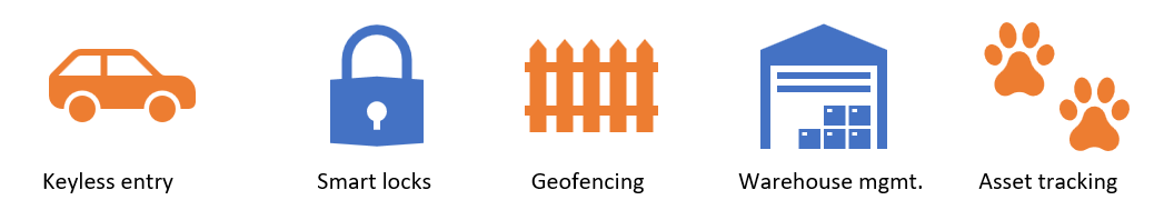
CS can be used for the following use cases:
- Keyless vehicle entry, performed by communication between a key fob or phone and the car’s anchor points
- Smart locks, to permit access only when an authorized device is within a designated proximity to the locks
- Geofencing, to limit access to designated areas
- Warehouse management, to monitor inventory and manage logistics
- Asset tracking for virtually any object of interest
In the past, Bluetooth devices would use a received signal strength indicator (RSSI) measurement to infer the distance between two of them. They would assume a free space path loss on the link, and use a straightforward equation to estimate distance:
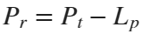
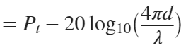
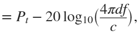 where
whereSo in this method, 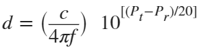 . But if the signal suffers more loss from multipath or shadowing, then the distance would be overestimated. Something better needed to be found.
. But if the signal suffers more loss from multipath or shadowing, then the distance would be overestimated. Something better needed to be found.Bluetooth 6.0 introduces not one, but two ways to accurately measure distance:
- Round-trip time (RTT) measurement
- Phase-based ranging (PBR) measurement
The RTT measurement method uses the fact that the Bluetooth signal time of flight (TOF) between two devices is half the RTT. It can then accurately compute the distance d as
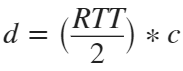 , where c is again the speed of light. This method requires accurate measurements of the time of departure (TOD) of the outbound signal from device 1 (the Initiator), time of arrival (TOA) of the outbound signal to device 2 (the Reflector), TOD of the return signal from device 2, and TOA of the return signal to device 1. The diagram below shows the signal paths and the times.
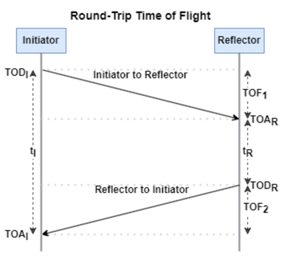
If you want to see how you can use MATLAB to simulate the RTT method, take a look at Estimate Distance Between Bluetooth LE Devices by Using Channel Sounding and Round-Trip Timing.
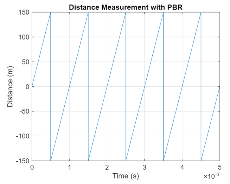
The PBR method uses two Bluetooth signals of different frequencies to measure distance. These signals are simply tones – sine waves. Without going through the derivation, PBR calculates distance d as
The mod() operation is needed to eliminate ambiguities in the distance calculation and the final division by two is to convert a round trip distance to a one-way distance. Because a given phase difference value can hold true for an infinite number of distance values, the mod() operation chooses the smallest distance that satisfies the equation. Also, these tones can be as close as 1 MHz apart. In that case, the maximum resolvable distance measurement is about 150 m. The plot below shows that ambiguity and repetition in distance measurement.
If you want to see how you can use MATLAB to simulate the PBR method, take a look at Estimate Distance Between Bluetooth LE Devices by Using Channel Sounding and Phase-Based Ranging.
Bluetooth 6.0 outlines RTT and PBR distance measurement methods, but CS does not mandate a specific algorithm for calculating distance estimates. This flexibility allows device manufacturers to tailor solutions to various use cases, balancing computational complexity with required accuracy and adapting to different radio environments. Examples include simple phase difference calculations and FFT-based methods.
Although Bluetooth 6.0 is now out, it is far from a finished version. The SIG is actively working through the ratification process for two major extensions:
- High Data Throughput, up to 8 Mbps
- 5 and 6 GHz operation
See the last few minutes of this video from the SIG to learn more about these exciting future developments. And if you want to see more Bluetooth blogs, give a review of this one! Finally, if you have specific Bluetooth questions, give me a shout and let’s start a discussion!
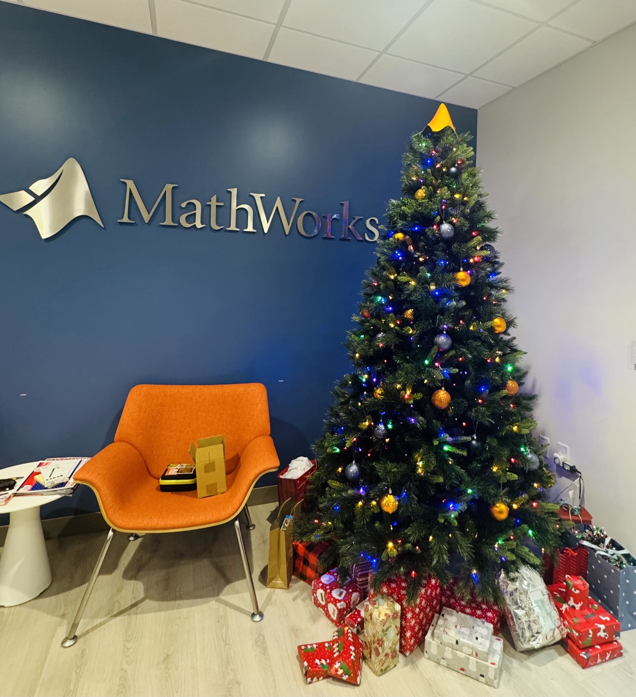
Christmas season is underway at my house:
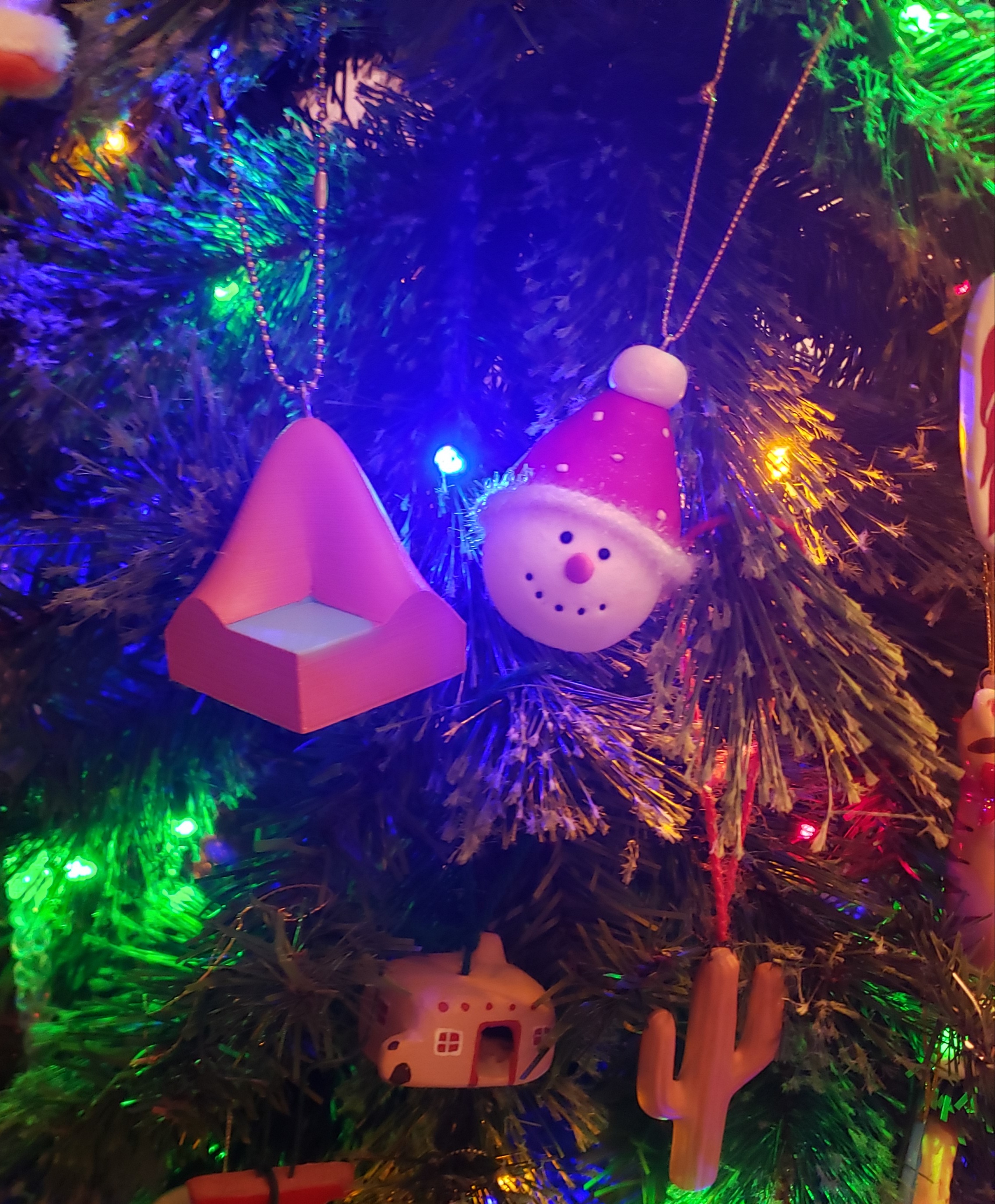
(Sorry - the ornament is not available at the MathWorks Merch Shop -- I made it with a 3-D printer.)
So I made this.
clear
close all
clc
% inspired from: https://www.youtube.com/watch?v=3CuUmy7jX6k
%% user parameters
h = 768;
w = 1024;
N_snowflakes = 50;
%% set figure window
figure(NumberTitle="off", ...
name='Mat-snowfalling-lab (right click to stop)', ...
MenuBar="none")
ax = gca;
ax.XAxisLocation = 'origin';
ax.YAxisLocation = 'origin';
axis equal
axis([0, w, 0, h])
ax.Color = 'k';
ax.XAxis.Visible = 'off';
ax.YAxis.Visible = 'off';
ax.Position = [0, 0, 1, 1];
%% first snowflake
ht = gobjects(1, 1);
for i=1:length(ht)
ht(i) = hgtransform();
ht(i).UserData = snowflake_factory(h, w);
ht(i).Matrix(2, 4) = ht(i).UserData.y;
ht(i).Matrix(1, 4) = ht(i).UserData.x;
im = imagesc(ht(i), ht(i).UserData.img);
im.AlphaData = ht(i).UserData.alpha;
colormap gray
end
%% falling snowflake
tic;
while true
% add a snowflake every 0.3 seconds
if toc > 0.3
if length(ht) < N_snowflakes
ht = [ht; hgtransform()];
ht(end).UserData = snowflake_factory(h, w);
ht(end).Matrix(2, 4) = ht(end).UserData.y;
ht(end).Matrix(1, 4) = ht(end).UserData.x;
im = imagesc(ht(end), ht(end).UserData.img);
im.AlphaData = ht(end).UserData.alpha;
colormap gray
end
tic;
end
ax.CLim = [0, 0.0005]; % prevent from auto clim
% move snowflakes
for i = 1:length(ht)
ht(i).Matrix(2, 4) = ht(i).Matrix(2, 4) + ht(i).UserData.velocity;
end
if strcmp(get(gcf, 'SelectionType'), 'alt')
set(gcf, 'SelectionType', 'normal')
break
end
drawnow
% delete the snowflakes outside the window
for i = length(ht):-1:1
if ht(i).Matrix(2, 4) < -length(ht(i).Children.CData)
delete(ht(i))
ht(i) = [];
end
end
end
%% snowflake factory
function snowflake = snowflake_factory(h, w)
radius = round(rand*h/3 + 10);
sigma = radius/6;
snowflake.velocity = -rand*0.5 - 0.1;
snowflake.x = rand*w;
snowflake.y = h - radius/3;
snowflake.img = fspecial('gaussian', [radius, radius], sigma);
snowflake.alpha = snowflake.img/max(max(snowflake.img));
end
Is it possible to differenciate the input, output and in-between wires by colors?
I was curious to startup your new AI Chat playground.
The first screen that popped up made the statement:
"Please keep in mind that AI sometimes writes code and text that seems accurate, but isnt"
Can someone elaborate on what exactly this means with respect to your AI Chat playground integration with the Matlab tools?
Are there any accuracy metrics for this integration?
We are thrilled to announce the grand prize winners of our MATLAB Shorts Mini Hack contest! This year, we invited the MATLAB Graphics and Charting team, the authors of the MATLAB functions used in every entry, to be our judges. After careful consideration, they have selected the top three winners:
Judge comments: Realism & detailed comments; wowed us with Manta Ray
2nd place – Jenny Bosten
Judge comments: Topical hacks : Auroras & Wind turbine; beautiful landscapes & nightscapes
3rd place - Vasilis Bellos
Judge comments: Nice algorithms & extra comments; can’t go wrong with Pumpkins
Judge comments: Impressive spring & cubes!
In addition, after validating the votes, we are pleased to announce the top 10 participants on the leaderboard:
Congratulations to all! Your creativity and skills have inspired many of us to explore and learn new skills, and make this contest a big success!
Dear MATLAB contest enthusiasts,
Welcome to the third installment of our interview series with top contest participants! This time we had the pleasure of talking to our all-time rock star – @Jenny Bosten. Every one of her entries is a masterpiece, demonstrating a deep understanding of the relationship between mathematics and aesthetics. Even Cleve Moler, the original author of MATLAB, is impressed and wrote in his blog: "Her code for Time Lapse of Lake View to the West shows she is also a wizard of coordinate systems and color maps."
you to read it to learn more about Jenny’s journey, her creative process, and her favorite entries.
Question: Who would you like to see featured in our next interview? Let us know your thoughts in the comments!
It would be nice to have a function to shade between two curves. This is a common question asked on Answers and there are some File Exchange entries on it but it's such a common thing to want to do I think there should be a built in function for it. I'm thinking of something like
plotsWithShading(x1, y1, 'r-', x2, y2, 'b-', 'ShadingColor', [.7, .5, .3], 'Opacity', 0.5);
So we can specify the coordinates of the two curves, and the shading color to be used, and its opacity, and it would shade the region between the two curves where the x ranges overlap. Other options should also be accepted, like line with, line style, markers or not, etc. Perhaps all those options could be put into a structure as fields, like
plotsWithShading(x1, y1, options1, x2, y2, options2, 'ShadingColor', [.7, .5, .3], 'Opacity', 0.5);
the shading options could also (optionally) be a structure. I know it can be done with a series of other functions like patch or fill, but it's kind of tricky and not obvious as we can see from the number of questions about how to do it.
Does anyone else think this would be a convenient function to add?
您也可以从以下列表中选择网站:
美洲
- América Latina (Español)
- Canada (English)
- United States (English)
欧洲
- Belgium (English)
- Denmark (English)
- Deutschland (Deutsch)
- España (Español)
- Finland (English)
- France (Français)
- Ireland (English)
- Italia (Italiano)
- Luxembourg (English)
- Netherlands (English)
- Norway (English)
- Österreich (Deutsch)
- Portugal (English)
- Sweden (English)
- Switzerland
- United Kingdom(English)
亚太
- Australia (English)
- India (English)
- New Zealand (English)
- 中国
- 日本Japanese (日本語)
- 한국Korean (한국어)