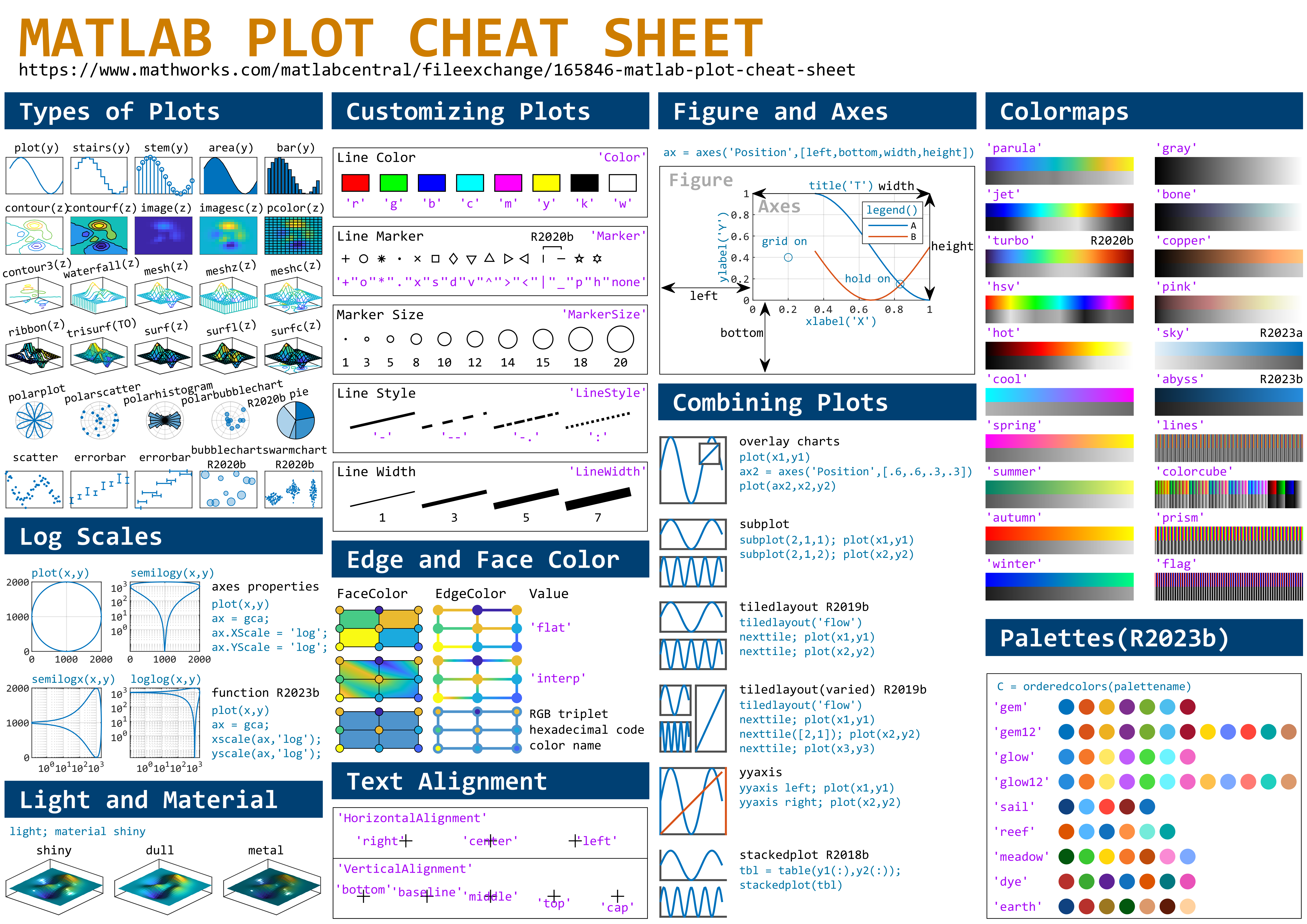
主要内容

Results for


If you've dabbled in "procedural generation," (algorithmically generating natural features), you may have come across the problem of sphere texturing. How to seamlessly texture a sphere is not immediately obvious. Watch what happens, for example, if you try adding power law noise to an evenly sampled grid of spherical angle coordinates (i.e. a "UV sphere" in Blender-speak):
% Example: how [not] to texture a sphere:
rng(2, 'twister'); % Make what I have here repeatable for you
% Make our radial noise, mapped onto an equal spaced longitude and latitude
% grid.
N = 51;
b = linspace(-1, 1, N).^2;
r = abs(ifft2(exp(6i*rand(N))./(b'+b+1e-5))); % Power law noise
r = rescale(r, 0, 1) + 5;
[lon, lat] = meshgrid(linspace(0, 2*pi, N), linspace(-pi/2, pi/2, N));
[x2, y2, z2] = sph2cart(lon, lat, r);
r2d = @(x)x*180/pi;
% Radial surface texture
subplot(1, 3, 1);
imagesc(r, 'Xdata', r2d(lon(1,:)), 'Ydata', r2d(lat(:, 1)));
xlabel('Longitude (Deg)');
ylabel('Latitude (Deg)');
title('Texture (radial variation)');
% View from z axis
subplot(1, 3, 2);
surf(x2, y2, z2, r);
axis equal
view([0, 90]);
title('Top view');
% Side view
subplot(1, 3, 3);
surf(x2, y2, z2, r);
axis equal
view([-90, 0]);
title('Side view');
The created surface shows "pinching" at the poles due to different radial values mapping to the same location. Furthermore, the noise statistics change based on the density of the sampling on the surface.
How can this be avoided? One standard method is to create a textured volume and sample the volume at points on a sphere. Code for doing this is quite simple:
rng default % Make our noise realization repeatable
% Create our 3D power-law noise
N = 201;
b = linspace(-1, 1, N);
[x3, y3, z3] = meshgrid(b, b, b);
b3 = x3.^2 + y3.^2 + z3.^2;
r = abs(ifftn(ifftshift(exp(6i*randn(size(b3)))./(b3.^1.2 + 1e-6))));
% Modify it - make it more interesting
r = rescale(r);
r = r./(abs(r - 0.5) + .1);
% Sample on a sphere
[x, y, z] = sphere(500);
% Plot
ir = interp3(x3, y3, z3, r, x, y, z, 'linear', 0);
surf(x, y, z, ir);
shading flat
axis equal off
set(gcf, 'color', 'k');
colormap(gray);
The result of evaluating this code is a seamless, textured sphere with no discontinuities at the poles or variation in the spatial statistics of the noise texture:
But what if you want to smooth it or perform some other local texture modification? Smoothing the volume and resampling is not equivalent to smoothing the surficial features shown on the map above.
A more flexible alternative is to treat the samples on the sphere surface as a set of interconnected nodes that are influenced by adjacent values. Using this approach we can start by defining the set of nodes on a sphere surface. These can be sampled almost arbitrarily, though the noise statistics will vary depending on the sampling strategy.
One noise realisation I find attractive can be had by randomly sampling a sphere. Normalizing a point in N-dimensional space by its 2-norm projects it to the surface of an N-dimensional unit sphere, so randomly sampling a sphere can be done very easily using randn() and vecnorm():
N = 5e3; % Number of nodes on our sphere
g=randn(3,N); % Random 3D points around origin
p=g./vecnorm(g); % Projected to unit sphere
The next step is to find each point's "neighbors." The first step is to find the convex hull. Since each point is on the sphere, the convex hull will include each point as a vertex in the triangulation:
k=convhull(p');
In the above, k is an N x 3 set of indices where each row represents a unique triangle formed by a triplicate of points on the sphere surface. The vertices of the full set of triangles containing a point describe the list of neighbors to that point.
What we want now is a large, sparse symmetric matrix where the indices of the columns & rows represent the indices of the points on the sphere and the nth row (and/or column) contains non-zero entries at the indices corresponding to the neighbors of the nth point.
How to do this? You could set up a tiresome nested for-loop searching for all rows (triangles) in k that contain some index n, or you could directly index via:
c=@(x)sparse(k(:,x)*[1,1,1],k,1,N,N);
t=c(1)|c(2)|c(3);
The result is the desired sparse connectivity matrix: a matrix with non-zero entries defining neighboring points.
So how do we create a textured sphere with this connectivity matrix? We will use it to form a set of equations that, when combined with the concept of "regularization," will allow us to determine the properties of the randomness on the surface. Our regularizer will penalize the difference of the radial distance of a point and the average of its neighbors. To do this we replace the main diagonal with the negative of the sum of the off-diagonal components so that the rows and columns are zero-mean. This can be done via:
w=spdiags(-sum(t,2)+1,0,double(t));
Now we invoke a bit of linear algebra. Pretend x is an N-length vector representing the radial distance of each point on our sphere with the noise realization we desire. Y will be an N-length vector of "observations" we are going to generate randomly, in this case using a uniform distribution (because it has a bias and we want a non-zero average radius, but you can play around with different distributions than uniform to get different effects):
Y=rand(N,1);
and A is going to be our "transformation" matrix mapping x to our noisy observations:
Ax = Y
In this case both x and Y are N length vectors and A is just the identity matrix:
A = speye(N);
Y, however, doesn't create the noise realization we want. So in the equation above, when solving for x we are going to introduce a regularizer which is going to penalize unwanted behavior of x by some amount. That behavior is defined by the point-neighbor radial differences represented in matrix w. Our estimate of x can then be found using one of my favorite Matlab assets, the "\" operator:
smoothness = 10; % Smoothness penalty: higher is smoother
x = (A+smoothness*w'*w)\Y; % Solving for radii
The vector x now contains the radii with the specified noise realization for the sphere which can be created simply by multiplying x by p and plotting using trisurf:
p2 = p.*x';
trisurf(k,p2(1,:),p2(2,:),p2(3,:),'FaceC', 'w', 'EdgeC', 'none','AmbientS',0,'DiffuseS',0.6,'SpecularS',1);
light;
set(gca, 'color', 'k');
axis equal
The following images show what happens as you change the smoothness parameter using values [.1, 1, 10, 100] (left to right):
Now you know a couple ways to make a textured sphere: that's the starting point for having a lot of fun with basic procedural planet, moon, or astroid generation! Here's some examples of things you can create based on these general ideas:
The MATLAB command window isn't just for commands and outputs—it can also host interactive hyperlinks. These can serve as powerful shortcuts, enhancing the feedback you provide during code execution. Here are some hyperlinks I frequently use in fprintf statements, warnings, or error messages.
1. Open a website.
msg = "Could not download data from website.";
url = "https://blogs.mathworks.com/graphics-and-apps/";
hypertext = "Go to website"
fprintf(1,'%s <a href="matlab: web(''%s'') ">%s</a>\n',msg,url,hypertext);
Could not download data from website. Go to website
2. Open a folder in file explorer (Windows)
msg = "File saved to current directory.";
directory = cd();
hypertext = "[Open directory]";
fprintf(1,'%s <a href="matlab: winopen(''%s'') ">%s</a>\n',msg,directory,hypertext)
File saved to current directory. [Open directory]
3. Open a document (Windows)
msg = "Created database.csv.";
filepath = fullfile(cd,'database.csv');
hypertext = "[Open file]";
fprintf(1,'%s <a href="matlab: winopen(''%s'') ">%s</a>\n',msg,filepath,hypertext)
Created database.csv. [Open file]
4. Open an m-file and go to a specific line
msg = 'Go to';
file = 'streamline.m';
line = 51;
fprintf(1,'%s <a href="matlab: matlab.desktop.editor.openAndGoToLine(which(''%s''), %d); ">%s line %d</a>', msg, file, line, file, line);
5. Display more text
msg = 'Incomplete data detected.';
extendedInfo = '\tFilename: m32c4r28\n\tDate: 12/20/2014\n\tElectrode: (3,7)\n\tDepth: ???\n';
hypertext = '[Click for more info]';
warning('%s <a href="matlab: fprintf(''%s'') ">%s</a>', msg,extendedInfo,hypertext);
Warning: Incomplete data detected. [Click for more info]
<click>
  • Filename: m32c4r28
  • Date: 12/20/2014
  • Electrode: (3,7)
  • Depth: ???
6. Run a function
Similarly, you can also add hyperlinks in figures and apps
See code here in our community contest area. (author: @Zhaoxu Liu / slandarer)
And what do you do for Valentine's Day?
K
K
Last activity 2024-2-10

which technical support should I contact/ask for the published Simscape example?
To enlarge an array with more rows and/or columns, you can set the lower right index to zero. This will pad the matrix with zeros.
m = rand(2, 3) % Initial matrix is 2 rows by 3 columns
mCopy = m;
% Now make it 2 rows by 5 columns
m(2, 5) = 0
m = mCopy; % Go back to original matrix.
% Now make it 3 rows by 3 columns
m(3, 3) = 0
m = mCopy; % Go back to original matrix.
% Now make it 3 rows by 7 columns
m(3, 7) = 0
Hannah
Hannah
Last activity 2024-2-8

I have been procrastinating on schoolwork by looking at all the amazing designs created in the last MATLAB Flipbook Mini Hack! They are just amazing. The voting is over but what are y'all's personal favorites? Mine is the flapping butterfly, it is for sure a creation I plan to share with others in the future!
function dragon24
% Copyright (c) 2024, Zhaoxu Liu / slandarer
baseV=[ -.016,.822; -.074,.809; -.114,.781; -.147,.738; -.149,.687; -.150,.630;
-.157,.554; -.166,.482; -.176,.425; -.208,.368; -.237,.298; -.284,.216;
-.317,.143; -.338,.091; -.362,.037;-.382,-.006;-.420,-.051;-.460,-.084;
-.477,-.110;-.430,-.103;-.387,-.084;-.352,-.065;-.317,-.060;-.300,-.082;
-.331,-.139;-.359,-.201;-.385,-.262;-.415,-.342;-.451,-.418;-.494,-.510;
-.533,-.599;-.569,-.675;-.607,-.753;-.647,-.829;-.689,-.932;-.699,-.988;
-.639,-.905;-.581,-.809;-.534,-.717;-.489,-.642;-.442,-.543;-.393,-.447;
-.339,-.362;-.295,-.296;-.251,-.251;-.206,-.241;-.183,-.281;-.175,-.350;
-.156,-.434;-.136,-.521;-.128,-.594;-.103,-.677;-.083,-.739;-.067,-.813;-.039,-.852];
% 基础比例、上色方式数据
baseV=[0,.82;baseV;baseV(end:-1:1,:).*[-1,1];0,.82];
baseV=baseV-mean(baseV,1);
baseF=1:size(baseV,1);
baseY=baseV(:,2);
baseY=(baseY-min(baseY))./(max(baseY)-min(baseY));
N=30;
baseR=sin(linspace(pi/4,5*pi/6,N))./1.2;
baseR=[baseR',baseR'];baseR(1,:)=[1,1];
baseR(5,:)=[2,.6];
baseR(10,:)=[3.7,.4];
baseR(15,:)=[1.8,.6];
baseT=[zeros(N,1),ones(N,1)];
baseM=zeros(N,2);
baseD=baseM;
ratioT=@(Mat,t)Mat*[cos(t),sin(t);-sin(t),cos(t)];
% 配色数据
CList=[211,56,32;56,105,166;253,209,95]./255;
% CList=bone(4);CList=CList(2:4,:);
% CList=flipud(bone(3));
% CList=lines(3);
% CList=colorcube(3);
% CList=rand(3)
baseC1=CList(2,:)+baseY.*(CList(1,:)-CList(2,:));
baseC2=CList(3,:)+baseY.*(CList(1,:)-CList(3,:));
% 构建图窗
fig=figure('units','normalized','position',[.1,.1,.5,.8],...
'UserData',[98,121,32,115,108,97,110,100,97,114,101,114]);
axes('parent',fig,'NextPlot','add','Color',[0,0,0],...
'DataAspectRatio',[1,1,1],'XLim',[-6,6],'YLim',[-6,6],'Position',[0,0,1,1]);
% 构造龙每个部分句柄
dragonHdl(1)=patch('Faces',baseF,'Vertices',baseV,'FaceVertexCData',baseC1,'FaceColor','interp','EdgeColor','none','FaceAlpha',.95);disp(char(fig.UserData))
for i=2:N
dragonHdl(i)=patch('Faces',baseF,'Vertices',baseV.*baseR(i,:)-[0,i./2.5-.3],'FaceVertexCData',baseC2,'FaceColor','interp','EdgeColor','none','FaceAlpha',.7);
end
set(dragonHdl(5),'FaceVertexCData',baseC1,'FaceAlpha',.7)
set(dragonHdl(10),'FaceVertexCData',baseC1,'FaceAlpha',.7)
set(dragonHdl(15),'FaceVertexCData',baseC1,'FaceAlpha',.7)
for i=N:-1:1,uistack(dragonHdl(i),'top');end
for i=1:N
baseM(i,:)=mean(get(dragonHdl(i),'Vertices'),1);
end
baseD=diff(baseM(:,2));Pos=[0,2];
% 主循环及旋转、运动计算
set(gcf,'WindowButtonMotionFcn',@dragonFcn)
fps=8;
game=timer('ExecutionMode', 'FixedRate', 'Period',1/fps, 'TimerFcn', @dragonGame);
start(game)
% Copyright (c) 2023, Zhaoxu Liu / slandarer
set(gcf,'tag','co','CloseRequestFcn',@clo);
function clo(~,~)
stop(game);delete(findobj('tag','co'));clf;close
end
function dragonGame(~,~)
Dir=Pos-baseM(1,:);
Dir=Dir./norm(Dir);
baseT=(baseT(1:end,:)+[Dir;baseT(1:end-1,:)])./2;
baseT=baseT./(vecnorm(baseT')');
theta=atan2(baseT(:,2),baseT(:,1))-pi/2;
baseM(1,:)=baseM(1,:)+(Pos-baseM(1,:))./30;
baseM(2:end,:)=baseM(1,:)+[cumsum(baseD.*baseT(2:end,1)),cumsum(baseD.*baseT(2:end,2))];
for ii=1:N
set(dragonHdl(ii),'Vertices',ratioT(baseV.*baseR(ii,:),theta(ii))+baseM(ii,:))
end
end
function dragonFcn(~,~)
xy=get(gca,'CurrentPoint');
x=xy(1,1);y=xy(1,2);
Pos=[x,y];
Pos(Pos>6)=6;
Pos(Pos<-6)=6;
end
end
There will be a warning when we try to solve equations with piecewise:
syms x y
a = x+y;
b = 1.*(x > 0) + 2.*(x <= 0);
eqns = [a + b*x == 1, a - b == 2];
S = solve(eqns, [x y]);
% 错误使用 mupadengine/feval_internal
% System contains an equation of an unknown type.
%
% 出错 sym/solve (第 293 行)
% sol = eng.feval_internal('solve', eqns, vars, solveOptions);
%
% 出错 demo3 (第 5 行)
% S=solve(eqns,[x y]);
But I found that the solve function can include functions such as heaviside to indicate positive and negative:
syms x y
a = x+y;
b = floor(heaviside(x)) - 2*abs(2*heaviside(x) - 1) + 2*floor(-heaviside(x)) + 4;
eqns = [a + b*x == 1, a - b == 2];
S = solve(eqns, [x y])
% S =
% 包含以下字段的 struct:
%
% x: -3/2
% y: 11/2
The piecewise function is divided into two sections, which is so complex, so this work must be encapsulated as a function to complete:
function pwFunc=piecewiseSym(x,waypoint,func,pfunc)
% @author : slandarer
gSign=[1,heaviside(x-waypoint)*2-1];
lSign=[heaviside(waypoint-x)*2-1,1];
inSign=floor((gSign+lSign)/2);
onSign=1-abs(gSign(2:end));
inFunc=inSign.*func;
onFunc=onSign.*pfunc;
pwFunc=simplify(sum(inFunc)+sum(onFunc));
end
Function Introduction
  • x : Argument
  • waypoint : Segmentation point of piecewise function
  • func : Functions on each segment
  • pfunc : The value at the segmentation point
example
syms x
% x waypoint func pfunc
f=piecewiseSym(x,[-1,1],[-x-1,-x^2+1,(x-1)^3],[-x-1,(x-1)^3]);
For example, find the analytical solution of the intersection point between the piecewise function and f=0.4 and plot it:
syms x
% x waypoint func pfunc
f=piecewiseSym(x,[-1,1],[-x-1,-x^2+1,(x-1)^3],[-x-1,(x-1)^3]);
% solve
S=solve(f==.4,x)
% S =
%
% -7/5
% (2^(1/3)*5^(2/3))/5 + 1
% -15^(1/2)/5
% 15^(1/2)/5
% draw
xx=linspace(-2,2,500);
f=matlabFunction(f);
yy=f(xx);
plot(xx,yy,'LineWidth',2);
hold on
scatter(double(S),.4.*ones(length(S),1),50,'filled')
precedent
syms x y
a=x+y;
b=piecewiseSym(x,0,[2,1],2);
eqns = [a + b*x == 1, a - b == 2];
S=solve(eqns,[x y])
% S =
% 包含以下字段的 struct:
%
% x: -3/2
% y: 11/2
It is pretty easy to draw a cool heatmap for I have uploaded a tool to fileexchange:
t=0.2:0.01:3*pi;
hold on
plot(t,cos(t)./(1+t),'LineWidth',4)
plot(t,sin(t)./(1+t),'LineWidth',4)
plot(t,cos(t+pi/2)./(1+t+pi/2),'LineWidth',4)
plot(t,cos(t+pi)./(1+t+pi),'LineWidth',4)
ax=gca;
hLegend=legend();
pause(1e-16)
colorData = uint8([255, 150, 200, 100; ...
255, 100, 50, 200; ...
0, 50, 100, 150; ...
102, 150, 200, 50]);
set(ax.Backdrop.Face, 'ColorBinding','interpolated','ColorData',colorData);
set(hLegend.BoxFace,'ColorBinding','interpolated','ColorData',colorData)
I have written two tools and uploaded fileexchange, which allows us to easily draw chord diagrams:
chord chart 弦图
download:
demo:
dataMat=[2 0 1 2 5 1 2;
3 5 1 4 2 0 1;
4 0 5 5 2 4 3];
dataMat=dataMat+rand(3,7);
dataMat(dataMat<1)=0;
colName={'G1','G2','G3','G4','G5','G6','G7'};
rowName={'S1','S2','S3'};
CC=chordChart(dataMat,'rowName',rowName,'colName',colName);
CC=CC.draw();
CC.setFont('FontSize',17,'FontName','Cambria')
% 显示刻度和数值
% Displays scales and numeric values
CC.tickState('on')
CC.tickLabelState('on')
% 调节标签半径
% Adjustable Label radius
CC.setLabelRadius(1.4);
Digraph chord chart 有向弦图
download:
demo:
dataMat=randi([0,8],[6,6]);
% 添加标签名称
NameList={'CHORD','CHART','MADE','BY','SLANDARER','MATLAB'};
BCC=biChordChart(dataMat,'Label',NameList,'Arrow','on');
BCC=BCC.draw();
% 添加刻度
BCC.tickState('on')
% 修改字体,字号及颜色
BCC.setFont('FontName','Cambria','FontSize',17,'Color',[.2,.2,.2])
BCC.setLabelRadius(1.3);
BCC.tickLabelState('on')
How to create a legend as follows?
Principle Explanation - Graphic Objects
Hidden Properties of Legend are laid as follows
In most cases, legends are drawn using LineLoop and Quadrilateral:
Both of these basic graphic objects are drawn in groups of four points, and the general principle is as follows:
Of course, you can arrange the points in order, or set VertexIndices whitch means the vertex order to obtain the desired quadrilateral shape:
Other objects
Compared to objects that can only be grouped into four points, we also need to introduce more flexible objects. Firstly, LineStrip, a graphical object that draws lines in groups of two points:
And TriangleStrip is a set of three points that draw objects to fill triangles, for example, complex polygons can be filled with multiple triangles:
Principle Explanation - Create and Replace
Let's talk about how to construct basic graphic objects, which are all constructed using undisclosed and very low-level functions, such as LineStrip, not through:
  • LineStrip()
It is built through:
  • matlab.graphics.primitive.world.LineStrip()
After building the object, the following properties must be set to make the hidden object visible:
  • Layer
  • ColorBinding
  • ColorData
  • VertexData
  • PickableParts
The settings of these properties can refer to the original legend to form the object, which will not be elaborated here. You can also refer to the code I wrote.
Afterwards, set the newly constructed object's parent class as the Group parent class of the original component, and then hide the original component
newBoxEdgeHdl.Parent=oriBoxEdgeHdl.Parent;
oriBoxEdgeHdl.Visible='off';
The above is the entire process of component replacement, with two example codes written:
Semi transparent legend
function SPrettyLegend(lgd)
% Semitransparent rounded rectangle legend
% Copyright (c) 2023, Zhaoxu Liu / slandarer
% -------------------------------------------------------------------------
% Zhaoxu Liu / slandarer (2023). pretty legend
% (https://www.mathworks.com/matlabcentral/fileexchange/132128-pretty-legend),
% MATLAB Central File Exchange. 检索来源 2023/7/9.
% =========================================================================
if nargin<1
ax = gca;
lgd = get(ax,'Legend');
end
pause(1e-6)
Ratio = .1;
t1 = linspace(0,pi/2,4); t1 = t1([1,2,2,3,3,4]);
t2 = linspace(pi/2,pi,4); t2 = t2([1,2,2,3,3,4]);
t3 = linspace(pi,3*pi/2,4); t3 = t3([1,2,2,3,3,4]);
t4 = linspace(3*pi/2,2*pi,4); t4 = t4([1,2,2,3,3,4]);
XX = [1,1,1-Ratio+cos(t1).*Ratio,1-Ratio,Ratio,Ratio+cos(t2).*Ratio,...
0,0,Ratio+cos(t3).*Ratio,Ratio,1-Ratio,1-Ratio+cos(t4).*Ratio];
YY = [Ratio,1-Ratio,1-Ratio+sin(t1).*Ratio,1,1,1-Ratio+sin(t2).*Ratio,...
1-Ratio,Ratio,Ratio+sin(t3).*Ratio,0,0,Ratio+sin(t4).*Ratio];
% 圆角边框(border-radius)
oriBoxEdgeHdl = lgd.BoxEdge;
newBoxEdgeHdl = matlab.graphics.primitive.world.LineStrip();
newBoxEdgeHdl.AlignVertexCenters = 'off';
newBoxEdgeHdl.Layer = 'front';
newBoxEdgeHdl.ColorBinding = 'object';
newBoxEdgeHdl.LineWidth = 1;
newBoxEdgeHdl.LineJoin = 'miter';
newBoxEdgeHdl.WideLineRenderingHint = 'software';
newBoxEdgeHdl.ColorData = uint8([38;38;38;0]);
newBoxEdgeHdl.VertexData = single([XX;YY;XX.*0]);
newBoxEdgeHdl.Parent=oriBoxEdgeHdl.Parent;
oriBoxEdgeHdl.Visible='off';
% 半透明圆角背景(Semitransparent rounded background)
oriBoxFaceHdl = lgd.BoxFace;
newBoxFaceHdl = matlab.graphics.primitive.world.TriangleStrip();
Ind = [1:(length(XX)-1);ones(1,length(XX)-1).*(length(XX)+1);2:length(XX)];
Ind = Ind(:).';
newBoxFaceHdl.PickableParts = 'all';
newBoxFaceHdl.Layer = 'back';
newBoxFaceHdl.ColorBinding = 'object';
newBoxFaceHdl.ColorType = 'truecoloralpha';
newBoxFaceHdl.ColorData = uint8(255*[1;1;1;.6]);
newBoxFaceHdl.VertexData = single([XX,.5;YY,.5;XX.*0,0]);
newBoxFaceHdl.VertexIndices = uint32(Ind);
newBoxFaceHdl.Parent = oriBoxFaceHdl.Parent;
oriBoxFaceHdl.Visible = 'off';
end
Usage examples
clc; clear; close all
rng(12)
% 生成随机点(Generate random points)
mu = [2 3; 6 7; 8 9];
S = cat(3,[1 0; 0 2],[1 0; 0 2],[1 0; 0 1]);
r1 = abs(mvnrnd(mu(1,:),S(:,:,1),100));
r2 = abs(mvnrnd(mu(2,:),S(:,:,2),100));
r3 = abs(mvnrnd(mu(3,:),S(:,:,3),100));
% 绘制散点图(Draw scatter chart)
hold on
propCell = {'LineWidth',1.2,'MarkerEdgeColor',[.3,.3,.3],'SizeData',60};
scatter(r1(:,1),r1(:,2),'filled','CData',[0.40 0.76 0.60],propCell{:});
scatter(r2(:,1),r2(:,2),'filled','CData',[0.99 0.55 0.38],propCell{:});
scatter(r3(:,1),r3(:,2),'filled','CData',[0.55 0.63 0.80],propCell{:});
% 增添图例(Draw legend)
lgd = legend('scatter1','scatter2','scatter3');
lgd.Location = 'northwest';
lgd.FontSize = 14;
% 坐标区域基础修饰(Axes basic decoration)
ax=gca; grid on
ax.FontName = 'Cambria';
ax.Color = [0.9,0.9,0.9];
ax.Box = 'off';
ax.TickDir = 'out';
ax.GridColor = [1 1 1];
ax.GridAlpha = 1;
ax.LineWidth = 1;
ax.XColor = [0.2,0.2,0.2];
ax.YColor = [0.2,0.2,0.2];
ax.TickLength = [0.015 0.025];
% 隐藏轴线(Hide XY-Ruler)
pause(1e-6)
ax.XRuler.Axle.LineStyle = 'none';
ax.YRuler.Axle.LineStyle = 'none';
SPrettyLegend(lgd)
Heart shaped legend (exclusive to pie charts)
function pie2HeartLegend(lgd)
% Heart shaped legend for pie chart
% Copyright (c) 2023, Zhaoxu Liu / slandarer
% -------------------------------------------------------------------------
% Zhaoxu Liu / slandarer (2023). pretty legend
% (https://www.mathworks.com/matlabcentral/fileexchange/132128-pretty-legend),
% MATLAB Central File Exchange. 检索来源 2023/7/9.
% =========================================================================
if nargin<1
ax = gca;
lgd = get(ax,'Legend');
end
pause(1e-6)
% 心形曲线(Heart curve)
x = -1:1/100:1;
y1 = 0.6 * abs(x) .^ 0.5 + ((1 - x .^ 2) / 2) .^ 0.5;
y2 = 0.6 * abs(x) .^ 0.5 - ((1 - x .^ 2) / 2) .^ 0.5;
XX = [x, flip(x),x(1)]./3.4+.5;
YY = ([y1, y2,y1(1)]-.2)./2+.5;
Ind = [1:(length(XX)-1);2:length(XX)];
Ind = Ind(:).';
% 获取图例图标(Get Legend Icon)
lgdEntryChild = lgd.EntryContainer.NodeChildren;
iconSet = arrayfun(@(lgdEntryChild)lgdEntryChild.Icon.Transform.Children.Children,lgdEntryChild,UniformOutput=false);
% 基础边框句柄(Base Border Handle)
newEdgeHdl = matlab.graphics.primitive.world.LineStrip();
newEdgeHdl.AlignVertexCenters = 'off';
newEdgeHdl.Layer = 'front';
newEdgeHdl.ColorBinding = 'object';
newEdgeHdl.LineWidth = .8;
newEdgeHdl.LineJoin = 'miter';
newEdgeHdl.WideLineRenderingHint = 'software';
newEdgeHdl.ColorData = uint8([38;38;38;0]);
newEdgeHdl.VertexData = single([XX;YY;XX.*0]);
newEdgeHdl.VertexIndices = uint32(Ind);
% 基础多边形面句柄(Base Patch Handle)
newFaceHdl = matlab.graphics.primitive.world.TriangleStrip();
Ind = [1:(length(XX)-1);ones(1,length(XX)-1).*(length(XX)+1);2:length(XX)];
Ind = Ind(:).';
newFaceHdl.PickableParts = 'all';
newFaceHdl.Layer = 'middle';
newFaceHdl.ColorBinding = 'object';
newFaceHdl.ColorType = 'truecoloralpha';
newFaceHdl.ColorData = uint8(255*[1;1;1;.6]);
newFaceHdl.VertexData = single([XX,.5;YY,.5;XX.*0,0]);
newFaceHdl.VertexIndices = uint32(Ind);
% 替换图例图标(Replace Legend Icon)
for i = 1:length(iconSet)
oriEdgeHdl = iconSet{i}(1);
tNewEdgeHdl = copy(newEdgeHdl);
tNewEdgeHdl.ColorData = oriEdgeHdl.ColorData;
tNewEdgeHdl.Parent = oriEdgeHdl.Parent;
oriEdgeHdl.Visible = 'off';
oriFaceHdl = iconSet{i}(2);
tNewFaceHdl = copy(newFaceHdl);
tNewFaceHdl.ColorData = oriFaceHdl.ColorData;
tNewFaceHdl.Parent = oriFaceHdl.Parent;
oriFaceHdl.Visible = 'off';
end
end
Usage examples
clc; clear; close all
% 生成随机点(Generate random points)
X = [1 3 0.5 2.5 2];
pieHdl = pie(X);
% 修饰饼状图(Decorate pie chart)
colorList=[0.4941 0.5490 0.4118
0.9059 0.6510 0.3333
0.8980 0.6157 0.4980
0.8902 0.5137 0.4667
0.4275 0.2824 0.2784];
for i = 1:2:length(pieHdl)
pieHdl(i).FaceColor=colorList((i+1)/2,:);
pieHdl(i).EdgeColor=colorList((i+1)/2,:);
pieHdl(i).LineWidth=1;
pieHdl(i).FaceAlpha=.6;
end
for i = 2:2:length(pieHdl)
pieHdl(i).FontSize=13;
pieHdl(i).FontName='Times New Roman';
end
lgd=legend('FontSize',13,'FontName','Times New Roman','TextColor',[1,1,1].*.3);
pie2HeartLegend(lgd)
I recently discovered a 2-minute video that introduces MatGPT, and I believe it's a resource worth sharing. The creator highlights MatGPT's impressive capabilities by demonstrating how it tackles the classic Travelling Salesman Problem.
With more than 13,000 downloads on File Exchange, MatGPT is gaining traction among users. I strongly recommend taking it for a spin to experience its potential firsthand.
I found this list on Book Authority about the top MATLAB books: https://bookauthority.org/books/best-matlab-books
My favorite book is Accelerating MATLAB Performance - 1001 tips to speed up MATLAB programs. I always pick something up from the book that helps me out.
how accurate are the answers of the AI Playground regarding information that are not specifiyed in the documentation?
A key aspect to masting MATLAB Graphics is getting a hang of the MATLAB Graphics Object Hierarchy which is essentially the structure of MATLAB figures that is used in the rendering pipeline. The base object is the Graphics Root (see groot) which contains the Figure. The Figure contains Axes or other containers such as a Tiled Chart Layout (see tiledlayout). Then these Axes can contain graphics primatives (the objects that contain data and get rendered) such as Lines or Patches.
Every graphics object has two important properties, the "Parent" and "Children" properties which can be used to access other objects in the tree. This can be very useful when trying to customize a pre-built chart (such as adding grid lines to both axes in an eye diagram chart) or when trying to access the axes of a non-current figure via a primative (so "gca" doesn't help out).
One last Tip and Trick with this is that you can declare graphics primatives without putting them on or creating an Axes by setting the first input argument to "gobjects(0)" which is an empty array of placeholder graphics objects. Then, when you have an Axes to plot the primitive on and are ready to render it, you can set the "Parent" of the object to your new Axes.
For Example:
l = line(gobjects(0), 1:10, 1:10);
...
...
...
l.Parent = gca;
Practicing navigating and exploring this tree will help propel your understanding of plotting in MATLAB.