主要内容
Results for
I've noticed is that the highly rated fonts for coding (e.g. Fira Code, Inconsolata, etc.) seem to overlook one issue that is key for coding in Matlab. While these fonts make 0 and O, as well as the 1 and l easily distinguishable, the brackets are not. Quite often the curly bracket looks similar to the curved bracket, which can lead to mistakes when coding or reviewing code.
So I was thinking: Could Mathworks put together a team to review good programming fonts, and come up with their own custom font designed specifically and optimized for Matlab syntax?
Hello everyone, i hope you all are in good health. i need to ask you about the help about where i should start to get indulge in matlab. I am an electrical engineer but having experience of construction field. I am new here. Please do help me. I shall be waiting forward to hear from you. I shall be grateful to you. Need recommendations and suggestions from experienced members. Thank you.
I recently wrote up a document which addresses the solution of ordinary and partial differential equations in Matlab (with some Python examples thrown in for those who are interested). For ODEs, both initial and boundary value problems are addressed. For PDEs, it addresses parabolic and elliptic equations. The emphasis is on finite difference approaches and built-in functions are discussed when available. Theory is kept to a minimum. I also provide a discussion of strategies for checking the results, because I think many students are too quick to trust their solutions. For anyone interested, the document can be found at https://blanchard.neep.wisc.edu/SolvingDifferentialEquationsWithMatlab.pdf
Kindly link me to the Channel Modeling Group.
I read and compreheneded a paper on channel modeling "An Adaptive Geometry-Based Stochastic Model for Non-Isotropic MIMO Mobile-to-Mobile Channels" except the graphical results obtained from the MATLAB codes. I have tried to replicate the same graphs but to no avail from my codes. And I am really interested in the topic, i have even written to the authors of the paper but as usual, there is no reply from them. Kindly assist if possible.
Hi, I'm looking for sites where I can find coding & algorithms problems and their solutions. I'm doing this workshop in college and I'll need some problems to go over with the students and explain how Matlab works by solving the problems with them and then reviewing and going over different solution options. Does anyone know a website like that? I've tried looking in the Matlab Cody By Mathworks, but didn't exactly find what I'm looking for. Thanks in advance.
An option for 10th degree polynomials but no weighted linear least squares. Seriously? Jesse
What do you think about the NVIDIA's achivement of becoming the top giant of manufacturing chips, especially for AI world?

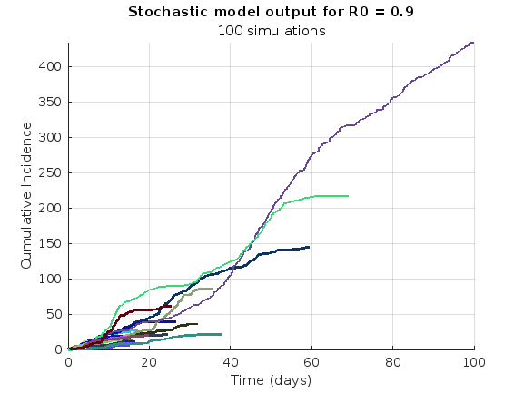
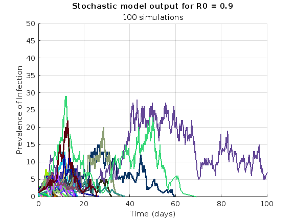
We are modeling the introduction of a novel pathogen into a completely susceptible population. In the cells below, I have provided you with the Matlab code for a simple stochastic SIR model, implemented using the "GillespieSSA" function
Simulating the stochastic model 100 times for 
Since γ is 0.4 per day,  per day
% Define the parameters
beta = 0.36;
gamma = 0.4;
n_sims = 100;
tf = 100; % Time frame changed to 100
% Calculate R0
R0 = beta / gamma
% Initial state values
initial_state_values = [1000000; 1; 0; 0]; % S, I, R, cum_inc
% Define the propensities and state change matrix
a = @(state) [beta * state(1) * state(2) / 1000000, gamma * state(2)];
nu = [-1, 0; 1, -1; 0, 1; 0, 0];
% Define the Gillespie algorithm function
function [t_values, state_values] = gillespie_ssa(initial_state, a, nu, tf)
t = 0;
state = initial_state(:); % Ensure state is a column vector
t_values = t;
state_values = state';
while t < tf
rates = a(state);
rate_sum = sum(rates);
if rate_sum == 0
break;
end
tau = -log(rand) / rate_sum;
t = t + tau;
r = rand * rate_sum;
cum_sum_rates = cumsum(rates);
reaction_index = find(cum_sum_rates >= r, 1);
state = state + nu(:, reaction_index);
% Update cumulative incidence if infection occurred
if reaction_index == 1
state(4) = state(4) + 1; % Increment cumulative incidence
end
t_values = [t_values; t];
state_values = [state_values; state'];
end
end
% Function to simulate the stochastic model multiple times and plot results
function simulate_stoch_model(beta, gamma, n_sims, tf, initial_state_values, R0, plot_type)
% Define the propensities and state change matrix
a = @(state) [beta * state(1) * state(2) / 1000000, gamma * state(2)];
nu = [-1, 0; 1, -1; 0, 1; 0, 0];
% Set random seed for reproducibility
rng(11);
% Initialize plot
figure;
hold on;
for i = 1:n_sims
[t, output] = gillespie_ssa(initial_state_values, a, nu, tf);
% Check if the simulation had only one step and re-run if necessary
while length(t) == 1
[t, output] = gillespie_ssa(initial_state_values, a, nu, tf);
end
if strcmp(plot_type, 'cumulative_incidence')
plot(t, output(:, 4), 'LineWidth', 2, 'Color', rand(1, 3));
elseif strcmp(plot_type, 'prevalence')
plot(t, output(:, 2), 'LineWidth', 2, 'Color', rand(1, 3));
end
end
xlabel('Time (days)');
if strcmp(plot_type, 'cumulative_incidence')
ylabel('Cumulative Incidence');
ylim([0 inf]);
elseif strcmp(plot_type, 'prevalence')
ylabel('Prevalence of Infection');
ylim([0 50]);
end
title(['Stochastic model output for R0 = ', num2str(R0)]);
subtitle([num2str(n_sims), ' simulations']);
xlim([0 tf]);
grid on;
hold off;
end
% Simulate the model 100 times and plot cumulative incidence
simulate_stoch_model(beta, gamma, n_sims, tf, initial_state_values, R0, 'cumulative_incidence');
% Simulate the model 100 times and plot prevalence
simulate_stoch_model(beta, gamma, n_sims, tf, initial_state_values, R0, 'prevalence');
Twitch built an entire business around letting you watch over someone's shoulder while they play video games. I feel like we should be able to make at least a few videos where we get to watch over someone's shoulder while they solve Cody problems. I would pay good money for a front-row seat to watch some of my favorite solvers at work. Like, I want to know, did Alfonso Nieto-Castonon just sit down and bang out some of those answers, or did he have to think about it for a while? What was he thinking about while he solved it? What resources was he drawing on? There's nothing like watching a master craftsman at work.
I can imagine a whole category of Cody videos called "How I Solved It". I tried making one of these myself a while back, but as far as I could tell, nobody else made one.
Here's the direct link to the video: https://www.youtube.com/watch?v=hoSmO1XklAQ
I hereby challenge you to make a "How I Solved It" video and post it here. If you make one, I'll make another one.
Base case:
Suppose you need to do a computation many times. We are going to assume that this computation cannot be vectorized. The simplest case is to use a for loop:
number_of_elements = 1e6;
test_fcn = @(x) sqrt(x) / x;
tic
for i = 1:number_of_elements
x(i) = test_fcn(i);
end
t_forward = toc;
disp(t_forward + " seconds")
Preallocation:
This can easily be sped up by preallocating the variable that houses results:
tic
x = zeros(number_of_elements, 1);
for i = 1:number_of_elements
x(i) = test_fcn(i);
end
t_forward_prealloc = toc;
disp(t_forward_prealloc + " seconds")
In this example, preallocation speeds up the loop by a factor of about three to four (running in R2024a). Comment below if you get dramatically different results.
disp(sprintf("%.1f", t_forward / t_forward_prealloc))
Run it in reverse:
Is there a way to skip the explicit preallocation and still be fast? Indeed, there is.
clear x
tic
for i = number_of_elements:-1:1
x(i) = test_fcn(i);
end
t_backward = toc;
disp(t_backward + " seconds")
By running the loop backwards, the preallocation is implicitly performed during the first iteration and the loop runs in about the same time (within statistical noise):
disp(sprintf("%.2f", t_forward_prealloc / t_backward))
Do you get similar results when running this code? Let us know your thoughts in the comments below.
Beneficial side effect:
Have you ever had to use a for loop to delete elements from a vector? If so, keeping track of index offsets can be tricky, as deleting any element shifts all those that come after. By running the for loop in reverse, you don't need to worry about index offsets while deleting elements.
The Ans Hack is a dubious way to shave a few points off your solution score. Instead of a standard answer like this
function y = times_two(x)
y = 2*x;
end
you would do this
function ans = times_two(x)
2*x;
end
The ans variable is automatically created when there is no left-hand side to an evaluated expression. But it makes for an ugly function. I don't think anyone actually defends it as a good practice. The question I would ask is: is it so offensive that it should be specifically disallowed by the rules? Or is it just one of many little hacks that you see in Cody, inelegant but tolerable in the context of the surrounding game?
Incidentally, I wrote about the Ans Hack long ago on the Community Blog. Dealing with user-unfriendly code is also one of the reasons we created the Head-to-Head voting feature. Some techniques are good for your score, and some are good for your code readability. You get to decide with you care about.
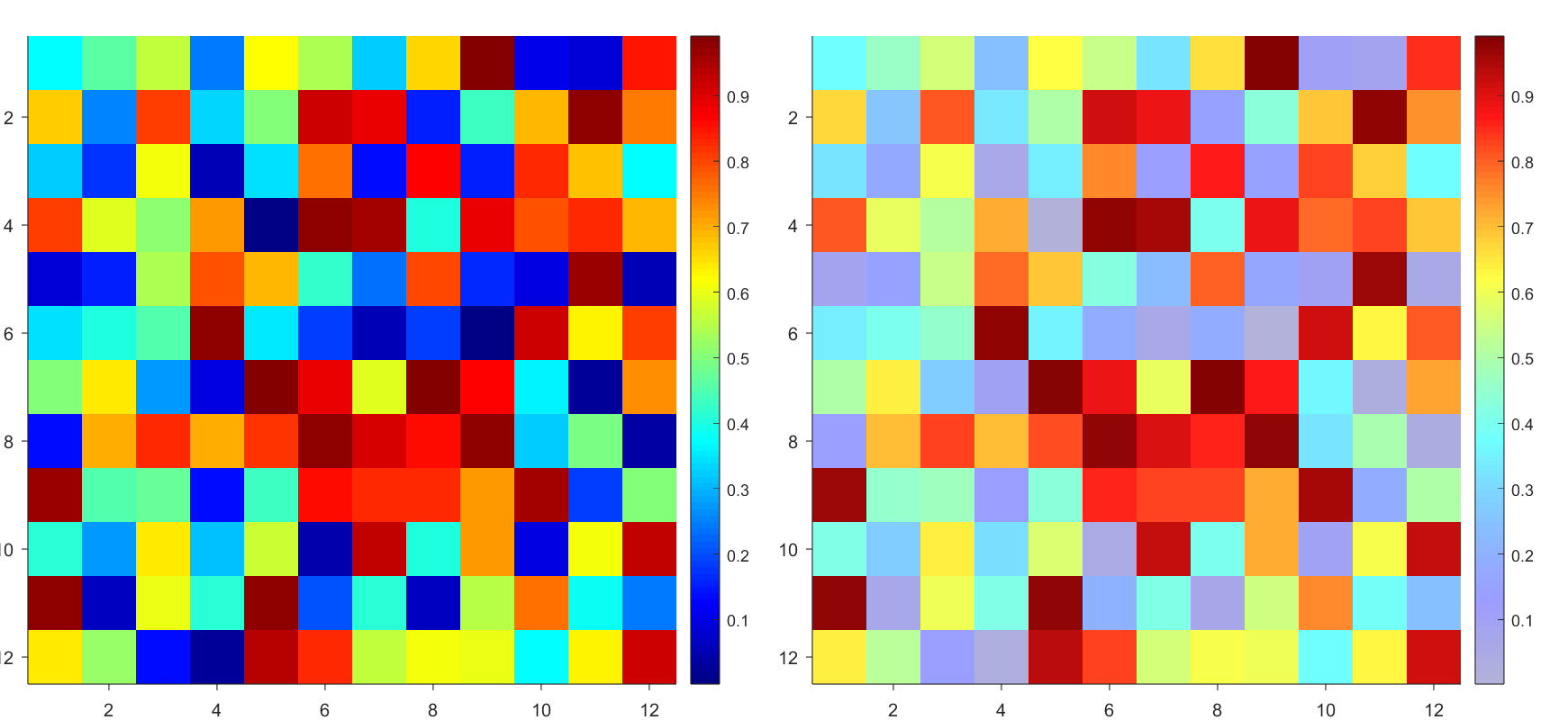
Many times when ploting, we not only need to set the color of the plot, but also its
transparency, Then how we set the alphaData of colorbar at the same time ?
It seems easy to do so :
data = rand(12,12);
% Transparency range 0-1, .3-1 for better appearance here
AData = rescale(- data, .3, 1);
% Draw an imagesc with numerical control over colormap and transparency
imagesc(data, 'AlphaData',AData);
colormap(jet);
ax = gca;
ax.DataAspectRatio = [1,1,1];
ax.TickDir = 'out';
ax.Box = 'off';
% get colorbar object
CBarHdl = colorbar;
pause(1e-16)
% Modify the transparency of the colorbar
CData = CBarHdl.Face.Texture.CData;
ALim = [min(min(AData)), max(max(AData))];
CData(4,:) = uint8(255.*rescale(1:size(CData, 2), ALim(1), ALim(2)));
CBarHdl.Face.Texture.ColorType = 'TrueColorAlpha';
CBarHdl.Face.Texture.CData = CData;
But !!!!!!!!!!!!!!! We cannot preserve the changes when saving them as images :
It seems that when saving plots, the `Texture` will be refresh, but the `Face` will not :
however, object Face only have 4 colors to change(The four corners of a quadrilateral), how
can we set more colors ??
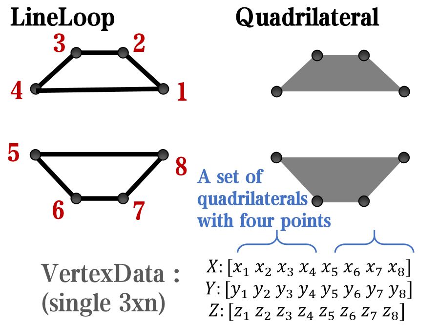
`Face` is a quadrilateral object, and we can change the `VertexData` to draw more than one little quadrilaterals:
data = rand(12,12);
% Transparency range 0-1, .3-1 for better appearance here
AData = rescale(- data, .3, 1);
%Draw an imagesc with numerical control over colormap and transparency
imagesc(data, 'AlphaData',AData);
colormap(jet);
ax = gca;
ax.DataAspectRatio = [1,1,1];
ax.TickDir = 'out';
ax.Box = 'off';
% get colorbar object
CBarHdl = colorbar;
pause(1e-16)
% Modify the transparency of the colorbar
CData = CBarHdl.Face.Texture.CData;
ALim = [min(min(AData)), max(max(AData))];
CData(4,:) = uint8(255.*rescale(1:size(CData, 2), ALim(1), ALim(2)));
warning off
CBarHdl.Face.ColorType = 'TrueColorAlpha';
VertexData = CBarHdl.Face.VertexData;
tY = repmat((1:size(CData,2))./size(CData,2), [4,1]);
tY1 = tY(:).'; tY2 = tY - tY(1,1); tY2(3:4,:) = 0; tY2 = tY2(:).';
tM1 = [tY1.*0 + 1; tY1; tY1.*0 + 1];
tM2 = [tY1.*0; tY2; tY1.*0];
CBarHdl.Face.VertexData = repmat(VertexData, [1,size(CData,2)]).*tM1 + tM2;
CBarHdl.Face.ColorData = reshape(repmat(CData, [4,1]), 4, []);
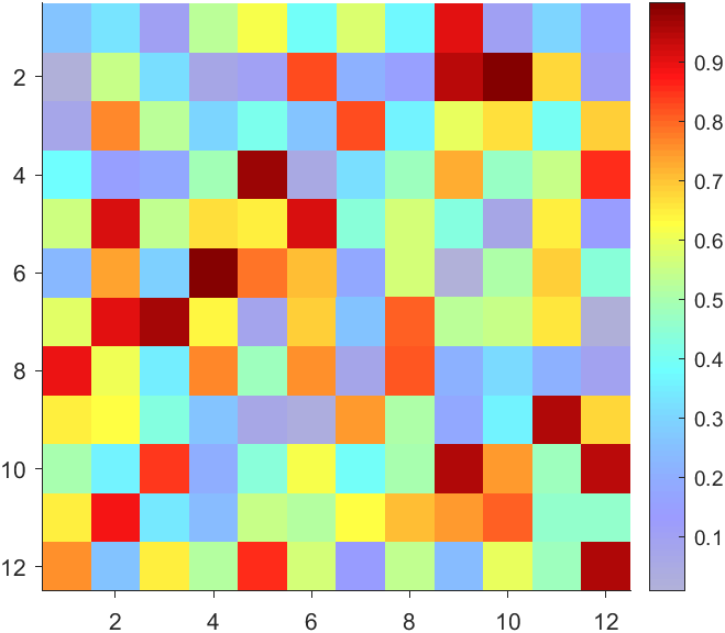
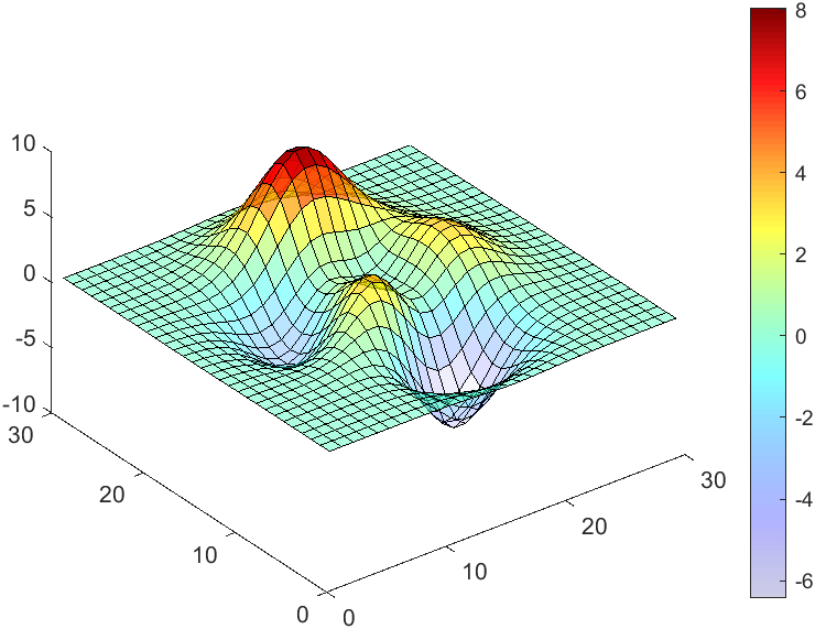
The higher the value, the more transparent it becomes
data = rand(12,12);
AData = rescale(- data, .3, 1);
imagesc(data, 'AlphaData',AData);
colormap(jet);
ax = gca;
ax.DataAspectRatio = [1,1,1];
ax.TickDir = 'out';
ax.Box = 'off';
CBarHdl = colorbar;
pause(1e-16)
CData = CBarHdl.Face.Texture.CData;
ALim = [min(min(AData)), max(max(AData))];
CData(4,:) = uint8(255.*rescale(size(CData, 2):-1:1, ALim(1), ALim(2)));
warning off
CBarHdl.Face.ColorType = 'TrueColorAlpha';
VertexData = CBarHdl.Face.VertexData;
tY = repmat((1:size(CData,2))./size(CData,2), [4,1]);
tY1 = tY(:).'; tY2 = tY - tY(1,1); tY2(3:4,:) = 0; tY2 = tY2(:).';
tM1 = [tY1.*0 + 1; tY1; tY1.*0 + 1];
tM2 = [tY1.*0; tY2; tY1.*0];
CBarHdl.Face.VertexData = repmat(VertexData, [1,size(CData,2)]).*tM1 + tM2;
CBarHdl.Face.ColorData = reshape(repmat(CData, [4,1]), 4, []);
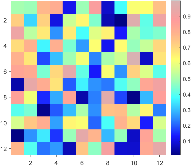
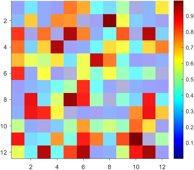
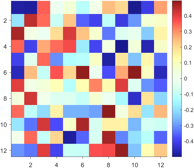
More transparent in the middle
data = rand(12,12) - .5;
AData = rescale(abs(data), .1, .9);
imagesc(data, 'AlphaData',AData);
colormap(jet);
ax = gca;
ax.DataAspectRatio = [1,1,1];
ax.TickDir = 'out';
ax.Box = 'off';
CBarHdl = colorbar;
pause(1e-16)
CData = CBarHdl.Face.Texture.CData;
ALim = [min(min(AData)), max(max(AData))];
CData(4,:) = uint8(255.*rescale(abs((1:size(CData, 2)) - (1 + size(CData, 2))/2), ALim(1), ALim(2)));
warning off
CBarHdl.Face.ColorType = 'TrueColorAlpha';
VertexData = CBarHdl.Face.VertexData;
tY = repmat((1:size(CData,2))./size(CData,2), [4,1]);
tY1 = tY(:).'; tY2 = tY - tY(1,1); tY2(3:4,:) = 0; tY2 = tY2(:).';
tM1 = [tY1.*0 + 1; tY1; tY1.*0 + 1];
tM2 = [tY1.*0; tY2; tY1.*0];
CBarHdl.Face.VertexData = repmat(VertexData, [1,size(CData,2)]).*tM1 + tM2;
CBarHdl.Face.ColorData = reshape(repmat(CData, [4,1]), 4, []);
The code will work if the plot have AlphaData property
data = peaks(30);
AData = rescale(data, .2, 1);
surface(data, 'FaceAlpha','flat','AlphaData',AData);
colormap(jet(100));
ax = gca;
ax.DataAspectRatio = [1,1,1];
ax.TickDir = 'out';
ax.Box = 'off';
view(3)
CBarHdl = colorbar;
pause(1e-16)
CData = CBarHdl.Face.Texture.CData;
ALim = [min(min(AData)), max(max(AData))];
CData(4,:) = uint8(255.*rescale(1:size(CData, 2), ALim(1), ALim(2)));
warning off
CBarHdl.Face.ColorType = 'TrueColorAlpha';
VertexData = CBarHdl.Face.VertexData;
tY = repmat((1:size(CData,2))./size(CData,2), [4,1]);
tY1 = tY(:).'; tY2 = tY - tY(1,1); tY2(3:4,:) = 0; tY2 = tY2(:).';
tM1 = [tY1.*0 + 1; tY1; tY1.*0 + 1];
tM2 = [tY1.*0; tY2; tY1.*0];
CBarHdl.Face.VertexData = repmat(VertexData, [1,size(CData,2)]).*tM1 + tM2;
CBarHdl.Face.ColorData = reshape(repmat(CData, [4,1]), 4, []);

The study of the dynamics of the discrete Klein - Gordon equation (DKG) with friction is given by the equation :

In the above equation, W describes the potential function:
to which every coupled unit  adheres. In Eq. (1), the variable $
 $ is the unknown displacement of the oscillator occupying the n-th position of the lattice, and
  is the discretization parameter. We denote by h the distance between the oscillators of the lattice. The chain (DKG) contains linear damping with a damping coefficient
  , while
 is the coefficient of the nonlinear cubic term.
$ is the unknown displacement of the oscillator occupying the n-th position of the lattice, and For the DKG chain (1), we will consider the problem of initial-boundary values, with initial conditions

and Dirichlet boundary conditions at the boundary points  and
and  , that is,
and , that is,
Therefore, when necessary, we will use the short notation  for the one-dimensional discrete Laplacian
for the one-dimensional discrete Laplacian
Now we want to investigate numerically the dynamics of the system (1)-(2)-(3). Our first aim is to conduct a numerical study of the property of Dynamic Stability of the system, which directly depends on the existence and linear stability of the branches of equilibrium points.
For the discussion of numerical results, it is also important to emphasize the role of the parameter  . By changing the time variable
  , we rewrite Eq. (1) in the form
 . We consider spatially extended initial conditions of the form:
We also assume zero initial velocity:
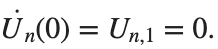
the following graphs for  and
and 
% Parameters
L = 200; % Length of the system
K = 99; % Number of spatial points
j = 2; % Mode number
omega_d = 1; % Characteristic frequency
beta = 1; % Nonlinearity parameter
delta = 0.05; % Damping coefficient
% Spatial grid
h = L / (K + 1);
n = linspace(-L/2, L/2, K+2); % Spatial points
N = length(n);
omegaDScaled = h * omega_d;
deltaScaled = h * delta;
% Time parameters
dt = 1; % Time step
tmax = 3000; % Maximum time
tspan = 0:dt:tmax; % Time vector
% Values of amplitude 'a' to iterate over
a_values = [2, 1.95, 1.9, 1.85, 1.82]; % Modify this array as needed
% Differential equation solver function
function dYdt = odefun(~, Y, N, h, omegaDScaled, deltaScaled, beta)
U = Y(1:N);
Udot = Y(N+1:end);
Uddot = zeros(size(U));
% Laplacian (discrete second derivative)
for k = 2:N-1
Uddot(k) = (U(k+1) - 2 * U(k) + U(k-1)) ;
end
% System of equations
dUdt = Udot;
dUdotdt = Uddot - deltaScaled * Udot + omegaDScaled^2 * (U - beta * U.^3);
% Pack derivatives
dYdt = [dUdt; dUdotdt];
end
% Create a figure for subplots
figure;
% Initial plot
a_init = 2; % Example initial amplitude for the initial condition plot
U0_init = a_init * sin((j * pi * h * n) / L); % Initial displacement
U0_init(1) = 0; % Boundary condition at n = 0
U0_init(end) = 0; % Boundary condition at n = K+1
subplot(3, 2, 1);
plot(n, U0_init, 'r.-', 'LineWidth', 1.5, 'MarkerSize', 10); % Line and marker plot
xlabel('$x_n$', 'Interpreter', 'latex');
ylabel('$U_n$', 'Interpreter', 'latex');
title('$t=0$', 'Interpreter', 'latex');
set(gca, 'FontSize', 12, 'FontName', 'Times');
xlim([-L/2 L/2]);
ylim([-3 3]);
grid on;
% Loop through each value of 'a' and generate the plot
for i = 1:length(a_values)
a = a_values(i);
% Initial conditions
U0 = a * sin((j * pi * h * n) / L); % Initial displacement
U0(1) = 0; % Boundary condition at n = 0
U0(end) = 0; % Boundary condition at n = K+1
Udot0 = zeros(size(U0)); % Initial velocity
% Pack initial conditions
Y0 = [U0, Udot0];
% Solve ODE
opts = odeset('RelTol', 1e-5, 'AbsTol', 1e-6);
[t, Y] = ode45(@(t, Y) odefun(t, Y, N, h, omegaDScaled, deltaScaled, beta), tspan, Y0, opts);
% Extract solutions
U = Y(:, 1:N);
Udot = Y(:, N+1:end);
% Plot final displacement profile
subplot(3, 2, i+1);
plot(n, U(end,:), 'b.-', 'LineWidth', 1.5, 'MarkerSize', 10); % Line and marker plot
xlabel('$x_n$', 'Interpreter', 'latex');
ylabel('$U_n$', 'Interpreter', 'latex');
title(['$t=3000$, $a=', num2str(a), '$'], 'Interpreter', 'latex');
set(gca, 'FontSize', 12, 'FontName', 'Times');
xlim([-L/2 L/2]);
ylim([-2 2]);
grid on;
end
% Adjust layout
set(gcf, 'Position', [100, 100, 1200, 900]); % Adjust figure size as needed
Dynamics for the initial condition ,  , for
, for  , for different amplitude values. By reducing the amplitude values, we observe the convergence to equilibrium points of different branches from
  and the appearance of values
  for which the solution converges to a non-linear equilibrium point
 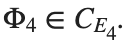 Parameters:
Detection of a stability threshold 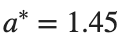 : For
: For  , the initial condition ,
 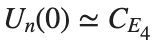 , converges to a non-linear equilibrium point
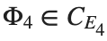 .
.
Characteristics for 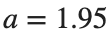 , with corresponding norm
 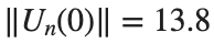 where the dynamics appear in the first image of the third row, we observe convergence to a non-linear equilibrium point of branch
  This has the same norm and the same energy as the previous case but the final state has a completely different profile. This result suggests secondary bifurcations have occurred in branch
where the dynamics appear in the first image of the third row, we observe convergence to a non-linear equilibrium point of branch By further reducing the amplitude, distinct values of  are discerned: 1.9, 1.85, 1.81 for which the initial condition
  with norms
 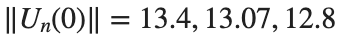 respectively, converges to a non-linear equilibrium point of branch
  This equilibrium point has norm
 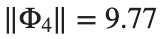 and energy
 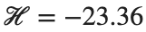 . The behavior of this equilibrium is illustrated in the third row and in the first image of the third row of Figure 1, and also in the first image of the third row of Figure 2. For all the values between the aforementioned a, the initial condition
  converges to geometrically different non-linear states of branch
  as shown in the second image of the first row and the first image of the second row of Figure 2, for amplitudes
 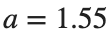 and
and 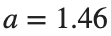 respectively.
respectively, converges to a non-linear equilibrium point of branch and energy Refference:
There are a host of problems on Cody that require manipulation of the digits of a number. Examples include summing the digits of a number, separating the number into its powers, and adding very large numbers together.
If you haven't come across this trick yet, you might want to write it down (or save it electronically):
digits = num2str(4207) - '0'
That code results in the following:
digits =
4 2 0 7
Now, summing the digits of the number is easy:
sum(digits)
ans =
13
Hello and a warm welcome to everyone! We're excited to have you in the Cody Discussion Channel. To ensure the best possible experience for everyone, it's important to understand the types of content that are most suitable for this channel.
Content that belongs in the Cody Discussion Channel:
- Tips & tricks: Discuss strategies for solving Cody problems that you've found effective.
- Ideas or suggestions for improvement: Have thoughts on how to make Cody better? We'd love to hear them.
- Issues: Encountering difficulties or bugs with Cody? Let us know so we can address them.
- Requests for guidance: Stuck on a Cody problem? Ask for advice or hints, but make sure to show your efforts in attempting to solve the problem first.
- General discussions: Anything else related to Cody that doesn't fit into the above categories.
Content that does not belong in the Cody Discussion Channel:
- Comments on specific Cody problems: Examples include unclear problem descriptions or incorrect testing suites.
- Comments on specific Cody solutions: For example, you find a solution creative or helpful.
Please direct such comments to the Comments section on the problem or solution page itself.
We hope the Cody discussion channel becomes a vibrant space for sharing expertise, learning new skills, and connecting with others.
Check out this episode about PIVLab: https://www.buzzsprout.com/2107763/15106425
Join the conversation with William Thielicke, the developer of PIVlab, as he shares insights into the world of particle image velocimetery (PIV) and its applications. Discover how PIV accurately measures fluid velocities, non invasively revolutionising research across the industries. Delve into the development journey of PI lab, including collaborations, key features and future advancements for aerodynamic studies, explore the advanced hardware setups camera technologies, and educational prospects offered by PIVlab, for enhanced fluid velocity measurements. If you are interested in the hardware he speaks of check out the company: Optolution.
One of the starter prompts is about rolling two six-sided dice and plot the results. As a hobby, I create my own board games. I was able to use the dice rolling prompt to show how a simple roll and move game would work. That was a great surprise!
How to leave feedback on a doc page
Leaving feedback is a two-step process. At the bottom of most pages in the MATLAB documentation is a star rating.

Start by selecting a star that best answers the question. After selecting a star rating, an edit box appears where you can offer specific feedback.
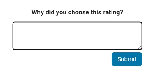
When you press "Submit" you'll see the confirmation dialog below. You cannot go back and edit your content, although you can refresh the page to go through that process again.

Tips on leaving feedback
- Be productive. The reader should clearly understand what action you'd like to see, what was unclear, what you think needs work, or what areas were really helpful.
- Positive feedback is also helpful. By nature, feedback often focuses on suggestions for changes but it also helps to know what was clear and what worked well.
- Point to specific areas of the page. This helps the reader to narrow the focus of the page to the area described by your feedback.
What happens to that feedback?
Before working at MathWorks I often left feedback on documentation pages but I never knew what happens after that. One day in 2021 I shared my speculation on the process:
> That feedback is received by MathWorks Gnomes which are never seen nor heard but visit the MathWorks documentation team at night while they are sleeping and whisper selected suggestions into their ears to manipulate their dreams. Occassionally this causes them to wake up with a Eureka moment that leads to changes in the documentation.

I'd like to let you in on the secret which is much less fanciful. Feedback left in the star rating and edit box are collected and periodically reviewed by the doc writers who look for trends on highly trafficked pages and finer grain feedback on less visited pages. Your feedback is important and often results in improvements.
Let's talk about probability theory in Matlab.
Conditions of the problem - how many more letters do I need to write to the sales department to get an answer?
To get closer to the problem, I need to buy a license under a contract. Maybe sometimes there are responsible employees sitting here who will give me an answer.
Thank you
In the MATLAB description of the algorithm for Lyapunov exponents, I believe there is ambiguity and misuse.
The lambda(i) in the reference literature signifies the Lyapunov exponent of the entire phase space data after expanding by i time steps, but in the calculation formula provided in the MATLAB help documentation, Y_(i+K) represents the data point at the i-th point in the reconstructed data Y after K steps, and this calculation formula also does not match the calculation code given by MATLAB. I believe there should be some misguidance and misunderstanding here.
According to the symbol regulations in the algorithm description and the MATLAB code, I think the correct formula might be y(i) = 1/dt * 1/N * sum_j( log( ||Y_(j+i) - Y_(j*+i)|| ) )
您也可以从以下列表中选择网站:
美洲
- América Latina (Español)
- Canada (English)
- United States (English)
欧洲
- Belgium (English)
- Denmark (English)
- Deutschland (Deutsch)
- España (Español)
- Finland (English)
- France (Français)
- Ireland (English)
- Italia (Italiano)
- Luxembourg (English)
- Netherlands (English)
- Norway (English)
- Österreich (Deutsch)
- Portugal (English)
- Sweden (English)
- Switzerland
- United Kingdom(English)
亚太
- Australia (English)
- India (English)
- New Zealand (English)
- 中国
- 日本Japanese (日本語)
- 한국Korean (한국어)