主要内容
Results for
Mathworks has always had quality documentation but in 2023, the documentation quality fell. Will this improve in 2024?
Hi
I have Matlab 2015b installed and if I try:
ones(2,3,4)+ones(2,3)
of course I get an error. But my student has R2023b installed and she gets a 2x3x4 matrix as a result, with all elements = 2.
How is it possible?
Thanks
A
Can you solve it?
This study explores the demographic patterns and disease outcomes during the cholera outbreak in London in 1849. Utilizing historical records and scholarly accounts, the research investigates the impact of the outbreak on the city' s population. While specific data for the 1849 cholera outbreak is limited, trends from similar 19th - century outbreaks suggest a high infection rate, potentially ranging from 30% to 50% of the population, owing to poor sanitation and overcrowded living conditions . Additionally, the birth rate in London during this period was estimated at 0.037 births per person per year . Although the exact reproduction number (R₀) for cholera in 1849 remains elusive, historical evidence implies a high R₀ due to the prevalent unsanitary conditions . This study sheds light on the challenges of estimating disease parameters from historical data, emphasizing the critical role of sanitation and public health measures in mitigating the impact of infectious diseases.
Introduction
The cholera outbreak of 1849 was a significant event in the history of cholera, a deadly waterborne disease caused by the bacterium Vibrio cholera. Cholera had several major outbreaks during the 19th century, and the one in 1849 was particularly devastating.
During this outbreak, cholera spread rapidly across Europe, including countries like England, France, and Germany . The disease also affected North America, with outbreaks reported in cities like New York and Montreal. The exact number of casualties from the 1849 cholera outbreak is difficult to determine due to limited record - keeping at that time. However, it is estimated that tens of thousands of people died as a result of the disease during this outbreak.
Cholera is highly contagious and spreads through contaminated water and food . The lack of proper sanitation and hygiene practices in the 19th century contributed to the rapid spread of the disease. It wasn't until the late 19th and early 20th centuries that advancements in public health, sanitation, and clean drinking water significantly reduced the incidence and impact of cholera outbreaks in many parts of the world.
Infection Rate
Based on general patterns observed in 19th - century cholera outbreaks and the conditions of that time, it' s reasonable to assume that the infection rate was quite high. During major cholera outbreaks in densely populated and unsanitary areas, infection rates could be as high as 30 - 50% or even more.
This means that in a densely populated city like London, with an estimated population of around 2.3 million in 1849, tens of thousands of people could have been infected during the outbreak. It' s important to emphasize that this is a rough estimation based on historical patterns and not specific to the 1849 outbreak. The actual infection rate could have varied widely based on the local conditions, public health measures in place, and the effectiveness of efforts to contain the disease.
For precise and localized estimations, detailed historical records specific to the 1849 cholera outbreak in a particular city or region would be required, and such data might not be readily available due to the limitations of historical documentation from that time period
Mortality Rate
It' s challenging to provide an exact death rate for the 1849 cholera outbreak because of the limited and often unreliable historical records from that time period. However, it is widely acknowledged that the death rate was significant, with tens of thousands of people dying as a result of the disease during this outbreak.
Cholera has historically been known for its high mortality rate, particularly in areas with poor sanitation and limited access to clean water. During cholera outbreaks in the 19th century, mortality rates could be extremely high, sometimes reaching 50% or more in affected communities. This high mortality rate was due to the rapid onset of severe dehydration and electrolyte imbalance caused by the cholera toxin, leading to death if not promptly treated.
Studies and historical accounts from various cholera outbreaks suggest that the R₀ for cholera can range from 1.5 to 2.5 or even higher in conditions where sanitation is inadequate and clean water is scarce. This means that one person with cholera could potentially infect 1.5 to 2.5 or more other people in such settings.
Unfortunately, there are no specific and reliable data available regarding the recovery rates from the 1849 cholera outbreak, as detailed and accurate record - keeping during that time period was limited. Cholera outbreaks in the 19th century were often devastating due to the lack of effective medical treatments and poor sanitation conditions. Recovery from cholera largely depended on the individual's ability to rehydrate, which was difficult given the rapid loss of fluids through severe diarrhea and vomiting .
LONDON CASE OF STUDY
In 1849, the estimated population of London was around 2.3 million people. London experienced significant population growth during the 19th century due to urbanization and industrialization. It’s important to note that historical population figures are often estimates, as comprehensive and accurate record-keeping methods were not as advanced as they are today.
% Define parameters
R0 = 2.5;
beta = 0.5;
gamma = 0.2; % Recovery rate
N = 2300000; % Total population
I0 = 1; % Initial number of infected individuals
% Define the SIR model differential equations
sir_eqns = @(t, Y) [-beta * Y(1) * Y(2) / N; % dS/dt
beta * Y(1) * Y(2) / N - gamma * Y(2); % dI/dt
gamma * Y(2)]; % dR/dt
% Initial conditions
Y0 = [N - I0; I0; 0]; % Initial conditions for S, I, R
% Time span
tmax1 = 100; % Define the maximum time (adjust as needed)
tspan = [0 tmax1];
% Solve the SIR model differential equations
[t, Y] = ode45(sir_eqns, tspan, Y0);
% Plot the results
figure;
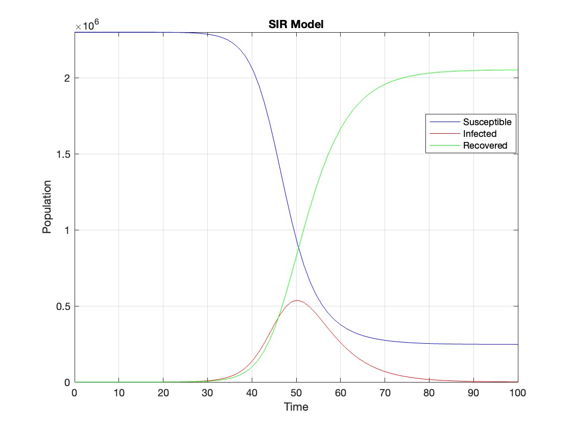
plot(t, Y(:,1), 'b', t, Y(:,2), 'r', t, Y(:,3), 'g');
legend('Susceptible', 'Infected', 'Recovered');
xlabel('Time');
ylabel('Population');
title('SIR Model');
axis tight;
grid on;
% Assuming t and Y are obtained from the ode45 solver for the SIR model
% Extract the infected population data (second column of Y)
infected = Y(:,2);
% Plot the infected population over time
figure;
plot(t, infected, 'r');
legend('Infected');
xlabel('Time');
ylabel('Population');
title('Infected Population over Time');
grid on;
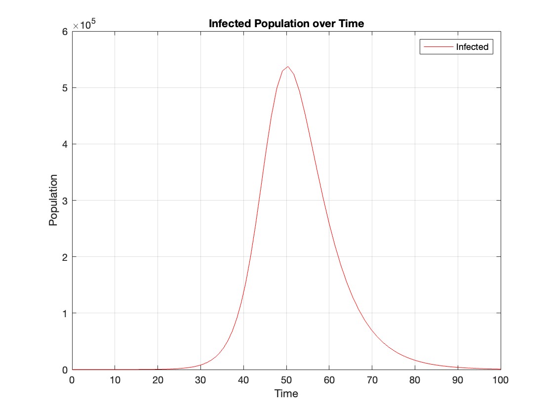
The code provides a visual representation of how the disease spreads and eventually diminishes within the population over the specified time interval . It can be used to understand the impact of different parameters (such as infection and recovery rates) on the progression of the outbreak .
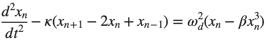
The study of nonlinear dynamical systems in lattices is an area of research with continuously growing interest.The first systematic studies of these systems emerged in the late 1930 s,thanks to the work of Frenkel and Kontorova on crystal dislocations.These studies led to the formulation of the discrete Klein-Gordon equation (DKG).Specifically,in 1939,Frenkel and Kontorova proposed a model that describes the structure and dynamics of a crystal lattice in a dislocation core.The FK model has become one of the fundamental models in physics,as it has been proven to reliably describe significant phenomena observed in discrete media.The equation we will examine is a variation of the following form:

The process described involves approximating a nonlinear differential equation through the Taylor method and simplifying it into a linear model.Let's analyze step by step the process from the initial equation to its final form.For small angles, can be approximated through the Taylor series as:
We substitute  in the original equation with the Taylor approximation:
To map this equation to a linear model,we consider the angles  to correspond to displacements
  in a mass-spring system.Thus,the equation transforms into:
to correspond to displacements We recognize that the term  expresses the nonlinearity of the system,while β is a coefficient corresponding to this nonlinearity,simplifying the expression.The final form of the equation is:
The exact value of β depends on the mapping of coefficients in the Taylor approximation and its application to the specific physical problem.Our main goal is to derive results regarding stability and convergence in nonlinear lattices under nonlinear conditions.We will examine the basic characteristics of the discrete Klein-Gordon equation:
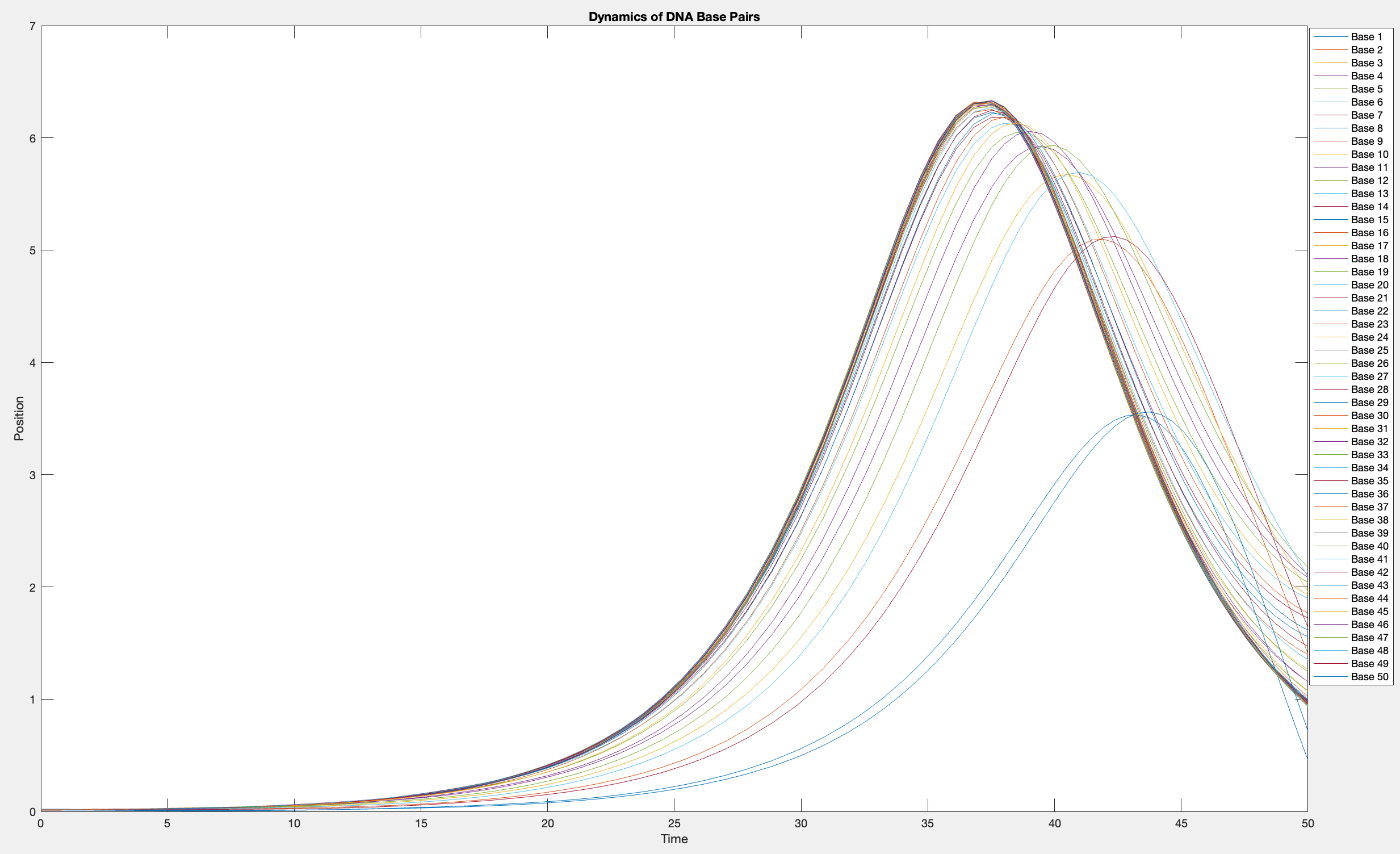
This model is often used to describe the opening of the DNA double helix during processes such as transcription.The model focuses on the transverse motion of the base pairs,which can be represented by a set of coupled nonlinear differential equations.
% Parameters
numBases = 50; % Number of base pairs
kappa = 0.1; % Elasticity constant
omegaD = 0.2; % Frequency term
beta = 0.05; % Nonlinearity coefficient
% Initial conditions
initialPositions = 0.01 + (0.02 - 0.01) * rand(numBases, 1);
initialVelocities = zeros(numBases, 1);
Time span
tSpan = [0 50];
>> % Differential equations
odeFunc = @(t, y) [y(numBases+1:end); ... % velocities
kappa * ([y(2); y(3:numBases); 0] - 2 * y(1:numBases) + [0; y(1:numBases-1)]) + ...
omegaD^2 * (y(1:numBases) - beta * y(1:numBases).^3)]; % accelerations
% Solve the system
[T, Y] = ode45(odeFunc, tSpan, [initialPositions; initialVelocities]);
% Visualization
plot(T, Y(:, 1:numBases))
legend(arrayfun(@(n) sprintf('Base %d', n), 1:numBases, 'UniformOutput', false))
xlabel('Time')
ylabel('Position')
title('Dynamics of DNA Base Pairs')
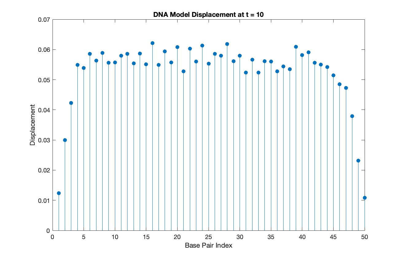
% Choose a specific time for the snapshot
snapshotTime = 10;
% Find the index in T that is closest to the snapshot time
[~, snapshotIndex] = min(abs(T - snapshotTime));
% Extract the solution at the snapshot time
snapshotSolution = Y(snapshotIndex, 1:numBases);
% Generate discrete plot for the DNA model at the snapshot time
figure;
stem(1:numBases, snapshotSolution, 'filled')
title(sprintf('DNA Model Displacement at t = %d', snapshotTime))
xlabel('Base Pair Index')
ylabel('Displacement')
% Time vector for detailed sampling
tDetailed = 0:0.5:50;
% Initialize an empty array to hold the data
data = [];
% Generate the data for 3D plotting
for i = 1:numBases
% Interpolate to get detailed solution data for each base pair
detailedSolution = interp1(T, Y(:, i), tDetailed);
% Concatenate the current base pair's data to the main data array
data = [data; repmat(i, length(tDetailed), 1), tDetailed', detailedSolution'];
end
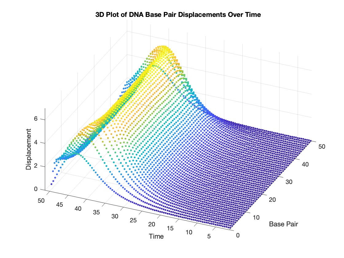
% 3D Plot
figure;
scatter3(data(:,1), data(:,2), data(:,3), 10, data(:,3), 'filled')
xlabel('Base Pair')
ylabel('Time')
zlabel('Displacement')
title('3D Plot of DNA Base Pair Displacements Over Time')
colormap('rainbow')
colorbar
Lots of students like me have a break from school this week or next! If y'all are looking for something interesting to do learn a bit about using hgtransform by making the transforming snake animation in MATLAB!
Code below!
⬇️⬇️⬇️
numblock=24;
v = [ -1 -1 -1 ; 1 -1 -1 ; -1 1 -1 ; -1 1 1 ; -1 -1 1 ; 1 -1 1 ];
f = [ 1 2 3 nan; 5 6 4 nan; 1 2 6 5; 1 5 4 3; 3 4 6 2 ];
clr = hsv(numblock);
shapes = [ 1 0 0 0 0 0 1 0 0 0 0 1 0 0 0 0 0 0 1 0 0 0 0 1 % box
0 0 .5 -.5 .5 0 1 0 -.5 .5 -.5 0 1 0 .5 -.5 .5 0 1 0 -.5 .5 -.5 0 % fluer
0 0 1 1 0 .5 -.5 1 .5 .5 -.5 -.5 1 .5 .5 -.5 -.5 1 .5 .5 -.5 -.5 1 .5 % bowl
0 .5 -.5 -.5 .5 -.5 .5 .5 -.5 .5 -.5 -.5 .5 -.5 .5 .5 -.5 .5 -.5 -.5 .5 -.5 .5 .5]; % ball
% Build the assembly
set(gcf,'color','black');
daspect(newplot,[1 1 1]);
xform=@(R)makehgtform('axisrotate',[0 1 0],R,'zrotate',pi/2,'yrotate',pi,'translate',[2 0 0]);
P=hgtransform('Parent',gca,'Matrix',makehgtform('xrotate',pi*.5,'zrotate',pi*-.8));
for i = 1:numblock
P = hgtransform('Parent',P,'Matrix',xform(shapes(end,i)*pi));
patch('Parent',P, 'Vertices', v, 'Faces', f, 'FaceColor',clr(i,:),'EdgeColor','none');
patch('Parent',P, 'Vertices', v*.75, 'Faces', f(end,:), 'FaceColor','none',...
'EdgeColor','w','LineWidth',2);
end
view([10 60]);
axis tight vis3d off
camlight
% Setup vectors for animation
h=findobj(gca,'type','hgtransform')'; h=h(2:end);
r=shapes(end,:)*pi;
steps=100;
% Animate between different shapes
for si = 1:size(shapes,1)
sh = shapes(si,:)*pi;
diff = (sh-r)/steps;
% Animate to a new shape
for s=1:steps
arrayfun(@(tx)set(h(tx),'Matrix',xform(r(tx)+diff(tx)*s)),1:numblock);
view([s*360/steps 20]); drawnow();
end
r=sh;
for s=1:steps; view([s*360/steps 20]); drawnow(); end % finish rotate
end
We are thrilled to announce the launch of a brand-new area within the MATLAB Central community – 'Discussions'. This exciting addition is designed to foster a stronger and more connected community.
Discover the 'Tips & Tricks' Channel
At the heart of 'Discussions' is the 'Tips & Tricks' channel. This is your ultimate destination for both sharing and discovering the best MATLAB tips.
Whether you're a seasoned MATLAB user with wisdom to share or a newcomer seeking advice, this channel is your platform. Here, you can post your own insights, ask for guidance on specific topics, and uncover hidden gems that can transform your MATLAB experience. It's more than just a channel; it's a community learning together; it’s your community blog!
More Than Just Tips
The 'Discussions' area offers much more. Explore the 'Ideas'channel to share and debate innovative product ideas. Dive into the 'Fun'channel to enjoy memes and light-hearted content with fellow MATLAB enthusiasts. Or wander into 'Off Topic'for intriguing discussions that might not be related to MATLAB.
Follow the channels!
We highly encourage every member of the MATLAB Central community to follow the channels you are interested in and participate in 'Discussions'. Together, we can achieve more, learn more, and connect more.

s = ['M','A','T','L','A','B']
9%
char([77,65,84,76,65,66])
7%
"MAT" + "LAB"
21%
upper(char('matlab' - '0' + 48))
17%
fliplr("BALTAM")
17%
rot90(rot90('BALTAM'))
30%
2929 个投票
The File Exchange team is thrilled to introduce a more streamlined approach to working with GitHub and File Exchange - the MATLAB and Simulink Integration for GitHub!
Key Enhancements:
- Improves the existing connection between File Exchange and GitHub, ensuring quicker reflection of changes made in GitHub within File Exchange.
- Aligns with GitHub's standard and supported approach to building integrations.
Action Required for File Exchange Contributors!
If you are a File Exchange contributor and have linked any submissions to GitHub, it is essential to install the App.
Starting April 16, 2024, your File Exchange submissions will no longer update automatically unless you take the following steps:
2. Follow the prompts on the page to install MATLAB and Simulink Integration for GitHub.

3. Complete the necessary steps in GitHub.
4. Return to the My File Exchange page and verify the installation.
If you prefer your File Exchange submission not to update automatically from GitHub, no action is required. Users will still be able to find and download your submissions. However, to release a new version of your code, you must either install the GitHub App or disconnect from GitHub and manually upload new versions of your code.
Should you have any questions or encounter issues with the App, please feel free to comment on this post!
Several of the colormaps are great for a 256 color surface plot, but aren't well optimized for extracting m colors for plotting several independent lines. The issue is that many colormaps have start/end colors that are too similar or are suboptimal colors for lines. There are certainly many workarounds for this, but it would be a great quality of life to adjust that directly when calling this.
Example:
x = linspace(0,2*pi,101)';
y = [1:6].*cos(x);
figure; plot(x,y,'LineWidth',2); grid on; axis tight;
And now if I wanted to color these lines, I could use something like turbo(6) or gray(6) and then apply it using colororder.
colororder(turbo(6))
But my issue is that the ends of the colormap are too similar. For other colormaps, you may get lines that are too light to be visible against the white background. There are plenty of workarounds, with my preference being to create extra colors and truncate that before using colororder.
cmap = turbo(8); cmap = cmap(2:end-1,:); % Truncate the end colors
figure; plot(x,y,'LineWidth',2); grid on; axis tight;
colororder(cmap)
I think it would be really awesome to add some name-argument input pair to these colormaps that can specify the range you want so this could even be done inside the colororder calling if desired. An example of my proposed solution would look something like this:
cmap = turbo(6,'Range',[0.1 0.8]); % Proposed idea to add functionality
Where in this scenario, the resulting colormap would be 6 equally spaced colors that range from 10% to 80% of the total color range. This would be especially nice because you could more quickly modify the range of colors, or you could set the limits regardless of whether you need to plot 3, 6, or 20 lines.
I asked my question in the general forum and a few minutes later it was deleted. Perhaps this is a better place?
Rather than using my German regional forum (as I do not speak German), I want to ask questions in an international English-speaking forum. Presumably there should be an international English forum for everyone around the world, as English is the first or second language of everyone who has gone to school. Where is it?
Big congratulations to @VBBV for achieving the remarkable milestone of 3,000 reputation points, earning the prestigious title of Editor within our community.
This achievement is a testament to @VBBV's exceptional contributions and steadfast commitment to the community. These efforts have also been endorsed by fellow top contributors, underscoring the value and impact of @VBBV's expertise.
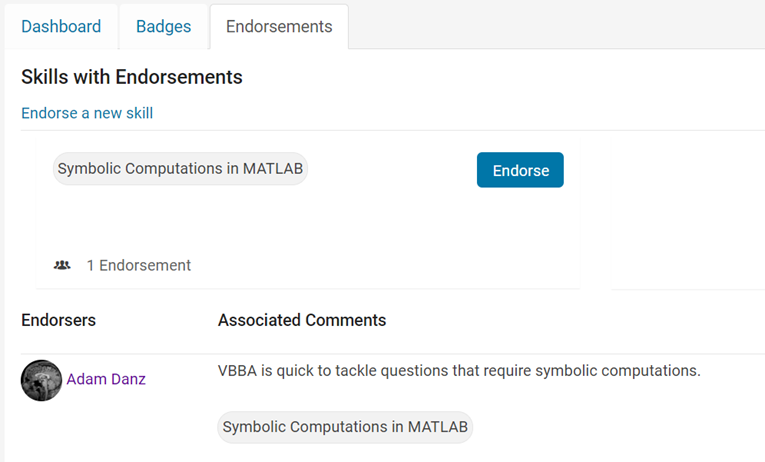
Welcome to the Editors' Club, @VBBV – we are excited to witness and support your continued journey and influence within our community!
eye(3) - diag(ones(1,3))
11%
0 ./ ones(3)
9%
cos(repmat(pi/2, [3,3]))
16%
zeros(3)
20%
A(3, 3) = 0
32%
mtimes([1;1;0], [0,0,0])
12%
3009 个投票
2 x 2 행렬의 행렬식은
- 행렬의 두 row 벡터로 정의되는 평행사변형의 면적입니다.
- 물론 두 column 벡터로 정의되는 평행사변형의 면적이기도 합니다.
- 좀 더 정확히는 signed area입니다. 면적이 음수가 될 수도 있다는 뜻이죠.
- 행렬의 두 행(또는 두 열)을 맞바꾸면 행렬식의 부호도 바뀌고 면적의 부호도 바뀌어야합니다.
일반적으로 n x n 행렬의 행렬식은
- 각 row 벡터(또는 각 column 벡터)로 정의되는 N차원 공간의 평행면체(?)의 signed area입니다.
- 제대로 이해하려면 대수학의 개념을 많이 가지고 와야 하는데 자세한 설명은 생략합니다.(=저도 모른다는 뜻)
- 더 자세히 알고 싶으시면 수학하는 만화의 '넓이 이야기' 편을 추천합니다.
- 수학적인 정의를 알고 싶으시면 위키피디아를 보시면 됩니다.
- 이렇게 생겼습니다. 좀 무섭습니다.
아래 코드는...
- 2 x 2 행렬에 대해서 이것을 수식 없이 그림만으로 증명하는 과정입니다.
- gif 생성에는 ScreenToGif를 사용했습니다. (gif 만들기엔 이게 킹왕짱인듯)
Determinant of 2 x 2 matrix is...
- An area of a parallelogram defined by two row vectors.
- Of course, same one defined by two column vectors.
- Precisely, a signed area, which means area can be negative.
- If two rows (or columns) are swapped, both the sign of determinant and area change.
More generally, determinant of n x n matrix is...
- Signed area of parallelepiped defined by rows (or columns) of the matrix in n-dim space.
- For a full understanding, a lot of concepts from abstract algebra should be brought, which I will not write here. (Cuz I don't know them.)
- For a mathematical definition of determinant, visit wikipedia.

- A little scary, isn't it?
The code below is...
- A process to prove the equality of the determinant of 2 x 2 matrix and the area of parallelogram.
- ScreenToGif is used to generate gif animation (which is, to me, the easiest way to make gif).
% 두 점 (a, b), (c, d)의 좌표
a = 4;
b = 1;
c = 1;
d = 3;
% patch 색 pre-define
lightgreen = [144, 238, 144]/255;
lightblue = [169, 190, 228]/255;
lightorange = [247, 195, 160]/255;
% animation params.
anim_Nsteps = 30;
% create window
figure('WindowStyle','docked')
ax = axes;
ax.XAxisLocation = 'origin';
ax.YAxisLocation = 'origin';
ax.XTick = [];
ax.YTick = [];
hold on
ax.XLim = [-.4, a+c+1];
ax.YLim = [-.4, b+d+1];
% create ad-bc patch
area = patch([0, a, a+c, c], [0, b, b+d, d], lightgreen);
p_ab = plot(a, b, 'ko', 'MarkerFaceColor', 'k');
p_cd = plot(c, d, 'ko', 'MarkerFaceColor', 'k');
p_ab.UserData = text(a+0.1, b, '(a, b)', 'FontSize',16);
p_cd.UserData = text(c+0.1, d-0.2, '(c, d)', 'FontSize',16);
area.UserData = text((a+c)/2-0.5, (b+d)/2, 'ad-bc', 'FontSize', 18);
pause
%% Is this really ad-bc?
area.UserData.String = 'ad-bc...?';
pause
%% fade out ad-bc
fadeinout(area, 0)
area.UserData.Visible = 'off';
pause
%% fade in ad block
rect_ad = patch([0, a, a, 0], [0, 0, d, d], lightblue, 'EdgeAlpha', 0, 'FaceAlpha', 0);
uistack(rect_ad, 'bottom');
fadeinout(rect_ad, 1, t_pause=0.003)
draw_gridline(rect_ad, ["23", "34"])
rect_ad.UserData = text(mean(rect_ad.XData), mean(rect_ad.YData), 'ad', 'FontSize', 20, 'HorizontalAlignment', 'center');
pause
%% fade-in bc block
rect_bc = patch([0, c, c, 0], [0, 0, b, b], lightorange, 'EdgeAlpha', 0, 'FaceAlpha', 0);
fadeinout(rect_bc, 1, t_pause=0.0035)
draw_gridline(rect_bc, ["23", "34"])
rect_bc.UserData = text(b/2, c/2, 'bc', 'FontSize', 20, 'HorizontalAlignment', 'center');
pause
%% slide ad block
patch_slide(rect_ad, ...
[0, 0, 0, 0], [0, b, b, 0], t_pause=0.004)
draw_gridline(rect_ad, ["12", "34"])
pause
%% slide ad block
patch_slide(rect_ad, ...
[0, 0, d/(d/c-b/a), d/(d/c-b/a)],...
[0, 0, b/a*d/(d/c-b/a), b/a*d/(d/c-b/a)], t_pause=0.004)
draw_gridline(rect_ad, ["14", "23"])
pause
%% slide bc block
uistack(p_cd, 'top')
patch_slide(rect_bc, ...
[0, 0, 0, 0], [d, d, d, d], t_pause=0.004)
draw_gridline(rect_bc, "34")
pause
%% slide bc block
patch_slide(rect_bc, ...
[0, 0, a, a], [0, 0, 0, 0], t_pause=0.004)
draw_gridline(rect_bc, "23")
pause
%% slide bc block
patch_slide(rect_bc, ...
[d/(d/c-b/a), 0, 0, d/(d/c-b/a)], ...
[b/a*d/(d/c-b/a), 0, 0, b/a*d/(d/c-b/a)], t_pause=0.004)
pause
%% finalize: fade out ad, bc, and fade in ad-bc
rect_ad.UserData.Visible = 'off';
rect_bc.UserData.Visible = 'off';
fadeinout([rect_ad, rect_bc, area], [0, 0, 1])
area.UserData.String = 'ad-bc';
area.UserData.Visible = 'on';
%% functions
function fadeinout(objs, inout, options)
arguments
objs
inout % 1이면 fade-in, 0이면 fade-out
options.anim_Nsteps = 30
options.t_pause = 0.003
end
for alpha = linspace(0, 1, options.anim_Nsteps)
for i = 1:length(objs)
switch objs(i).Type
case 'patch'
objs(i).FaceAlpha = (inout(i)==1)*alpha + (inout(i)==0)*(1-alpha);
objs(i).EdgeAlpha = (inout(i)==1)*alpha + (inout(i)==0)*(1-alpha);
case 'constantline'
objs(i).Alpha = (inout(i)==1)*alpha + (inout(i)==0)*(1-alpha);
end
pause(options.t_pause)
end
end
end
function patch_slide(obj, x_dist, y_dist, options)
arguments
obj
x_dist
y_dist
options.anim_Nsteps = 30
options.t_pause = 0.003
end
dx = x_dist/options.anim_Nsteps;
dy = y_dist/options.anim_Nsteps;
for i=1:options.anim_Nsteps
obj.XData = obj.XData + dx(:);
obj.YData = obj.YData + dy(:);
obj.UserData.Position(1) = mean(obj.XData);
obj.UserData.Position(2) = mean(obj.YData);
pause(options.t_pause)
end
end
function draw_gridline(patch, where)
ax = patch.Parent;
for i=1:length(where)
v1 = str2double(where{i}(1));
v2 = str2double(where{i}(2));
x1 = patch.XData(v1);
x2 = patch.XData(v2);
y1 = patch.YData(v1);
y2 = patch.YData(v2);
if x1==x2
xline(x1, 'k--')
else
fplot(@(x) (y2-y1)/(x2-x1)*(x-x1)+y1, [ax.XLim(1), ax.XLim(2)], 'k--')
end
end
end
Happy year of the dragon.
I was looking into the possibility of making a spin-to-win prize wheel in MATLAB. I was looking around, and if someone has made one before they haven't shared. A labeled colored spinning wheel, that would slow down and stop (or I would take just stopping) at a random spot each time. I would love any tips or links to helpful resources!
Greetings to all MATLAB users,
Although the MATLAB Flipbook contest has concluded, the pursuit of ‘learning while having fun’ continues. I would like to take this opportunity to highlight some recent insightful technical articles from a standout contest participant – Zhaoxu Liu / slandarer.
Zhaoxu has contributed eight informative articles to both the Tips & Tricks and Fun channels in our new Discussions area. His articles offer practical advice on topics such as customizing legends, constructing chord charts, and adding color to axes. Additionally, he has shared engaging content, like using MATLAB to create an interactive dragon that follows your mouse cursor, a nod to the upcoming Year of the Dragon in 2024!
I invite you to explore these articles for both enjoyment and education, and I hope you'll find new techniques to incorporate into your work.
Our community is full of individuals skilled in MATLAB, and we're always eager to learn from one another. Who would you like to see featured next? Or perhaps you have some tips & tricks of your own to contribute. Remember, sharing knowledge is a collaborative effort, as Confucius wisely stated, 'When I walk along with two others, they may serve me as my teachers.'
Let's maintain our commitment to a continuous learning journey. This could be the perfect warm-up for the upcoming 2024 contest.
Many of the examples in the MATLAB documentation are extremely high quality articles, often worthy of attention in their own right. Time to start celebrating them! Today's is how to increase Image Resolution using deep learning
https://uk.mathworks.com/help/deeplearning/ug/single-image-super-resolution-using-deep-learning.html
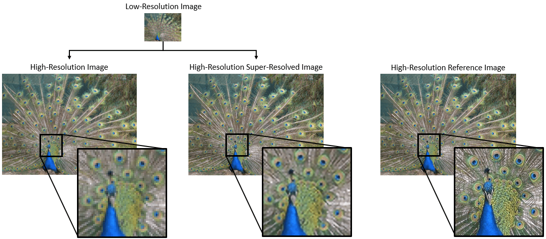
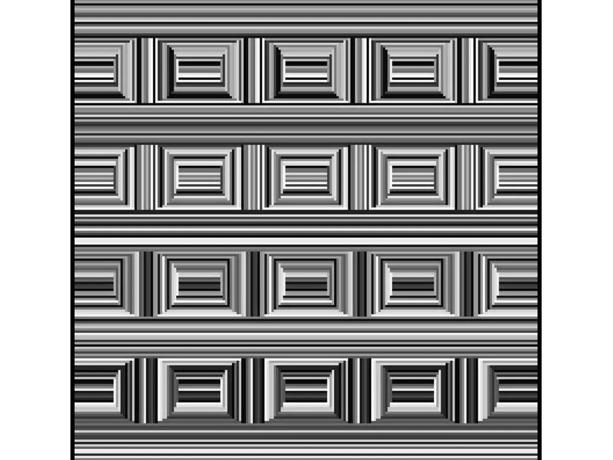
Can you see them?
I have been procrastinating on schoolwork by looking at all the amazing designs created in the last MATLAB Flipbook Mini Hack! They are just amazing. The voting is over but what are y'all's personal favorites? Mine is the flapping butterfly, it is for sure a creation I plan to share with others in the future!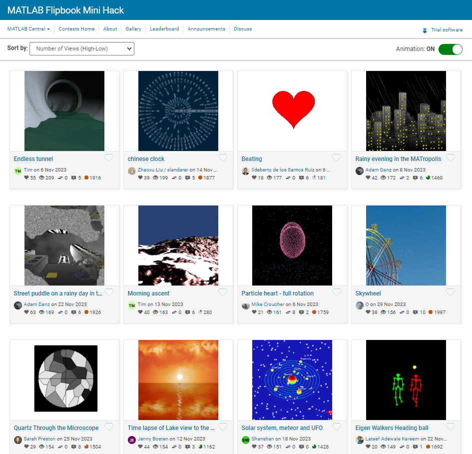
您也可以从以下列表中选择网站:
美洲
- América Latina (Español)
- Canada (English)
- United States (English)
欧洲
- Belgium (English)
- Denmark (English)
- Deutschland (Deutsch)
- España (Español)
- Finland (English)
- France (Français)
- Ireland (English)
- Italia (Italiano)
- Luxembourg (English)
- Netherlands (English)
- Norway (English)
- Österreich (Deutsch)
- Portugal (English)
- Sweden (English)
- Switzerland
- United Kingdom(English)
亚太
- Australia (English)
- India (English)
- New Zealand (English)
- 中国
- 日本Japanese (日本語)
- 한국Korean (한국어)