ans =
主要内容
搜索
This year's MATLAB Shorts Mini Hack contest has kicked off, and there are already lots of interesting entries. The contest features creating a 96-frame, 4-second animation, which is looped 3 times to compose a 12-second short movie. There is an option to add audio to enhance the animation, and it's restricted to a an upper limit of 2,000 characters to promote efficient coding.
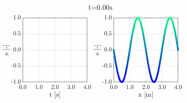
Many of the contestants have already realized the potential for creating a seamless loop, which provides a smooth transition and avoids any discontinuities when the animation is repeated. There are several ways to achieve this. An efficient method for example is utilizing sinusoidal functions, which are periodic, meaning that they repeat themselves over time:
An intuitive example of a seamless loop is @Edgar Guevara's EKG pulse entry, which features an electrocardiogram signal on an oscilloscope. The animation is perfectly matched by the audio, as explained in their post.
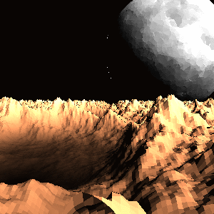
Another, rather sophisticated approach is featured in @Tim's Moonrun animation in last year's contest. This seamless loop is achieved by cleverly manipulating the camera position and target over a periodic spatial domain, producing this stunning result:
This essentially tells us that for a seamless loop in the spatial domain, the first frame must match the last frame (with a single timestep difference to be more precise, more on that later). But surely this cannot be achieved by zooming in, unless you are simulating a fractal. Well, there are always workarounds.
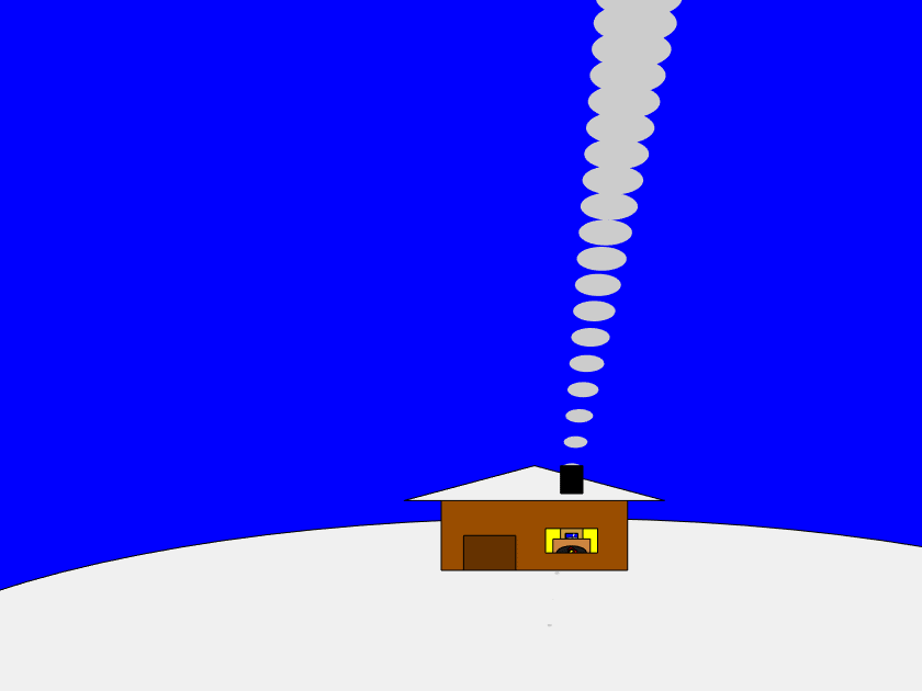
One way to achieve this is by zooming into a section that contains the first frame of the animation. This is featured in my Winter Loop entry. This is a remix of @Oliver Jaros's Winter entry, which was selected as a one of the weekly winners in the nature & space category for Week 1. The code was modified to lower the character count, but all credits for the original idea and graphics go to them. I also drew inspiration from one of my favourite games of all time, Super Mario 64. Oliver's animation reminded me of the Cool, Cool Mountain level of the game. In the game, you can enter various levels by jumping into paintings serving as portals.
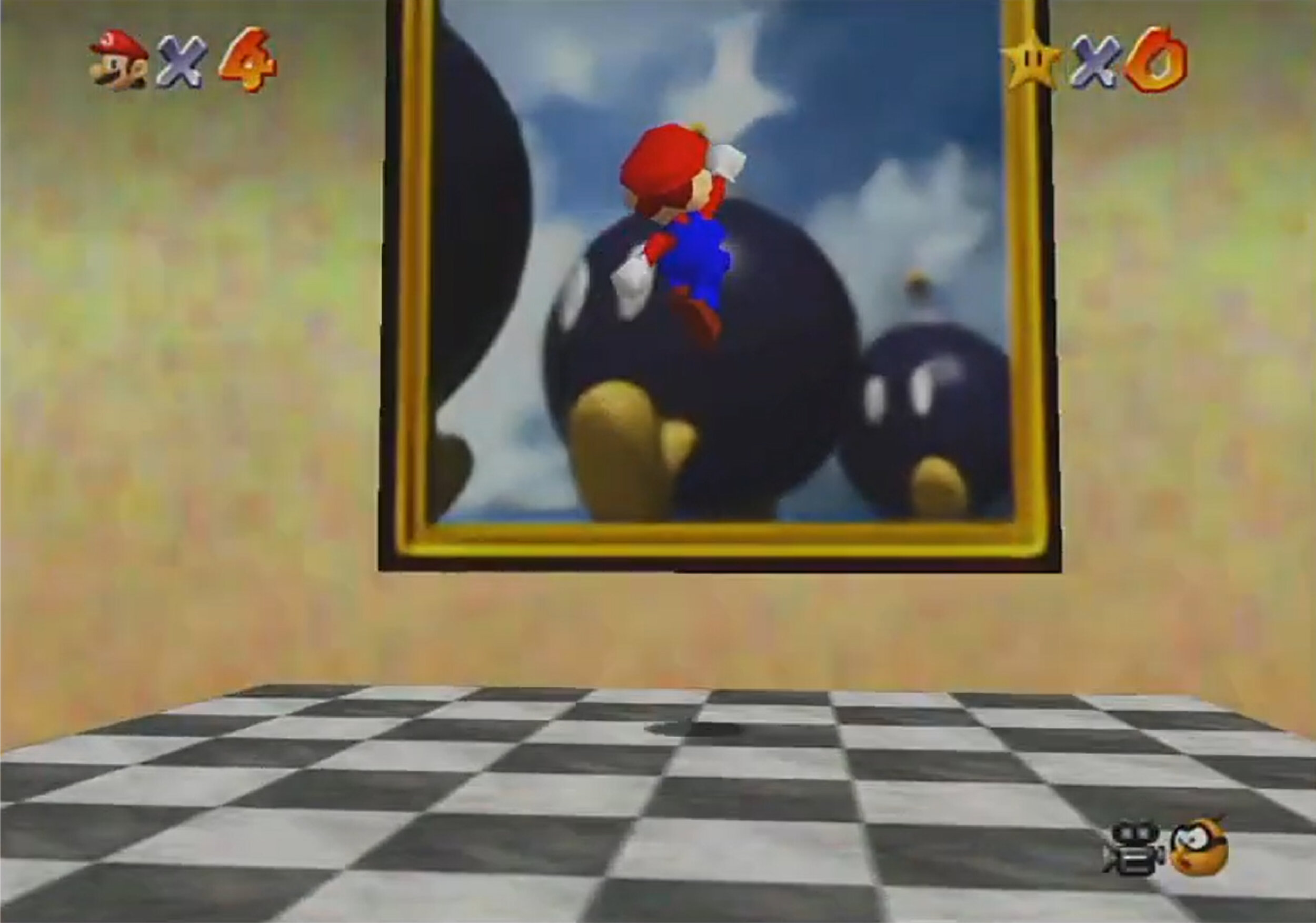
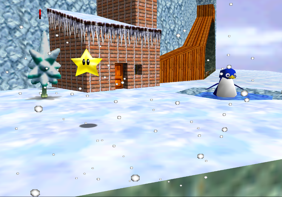
This inspired the idea of zooming into a rectangular photograph frame containing the first frame of the animation to facilitate restarting the loop. One could argue that it would probably take a crazy person to have a photo of their house framed inside their own house. Well, in this economy and with the current house prices, I don't think this scenario is too far-fetched:
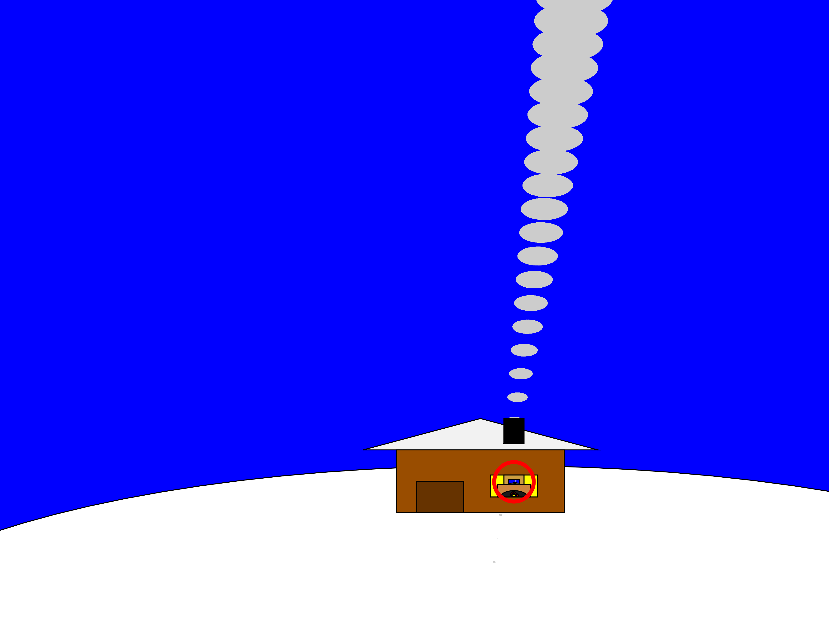
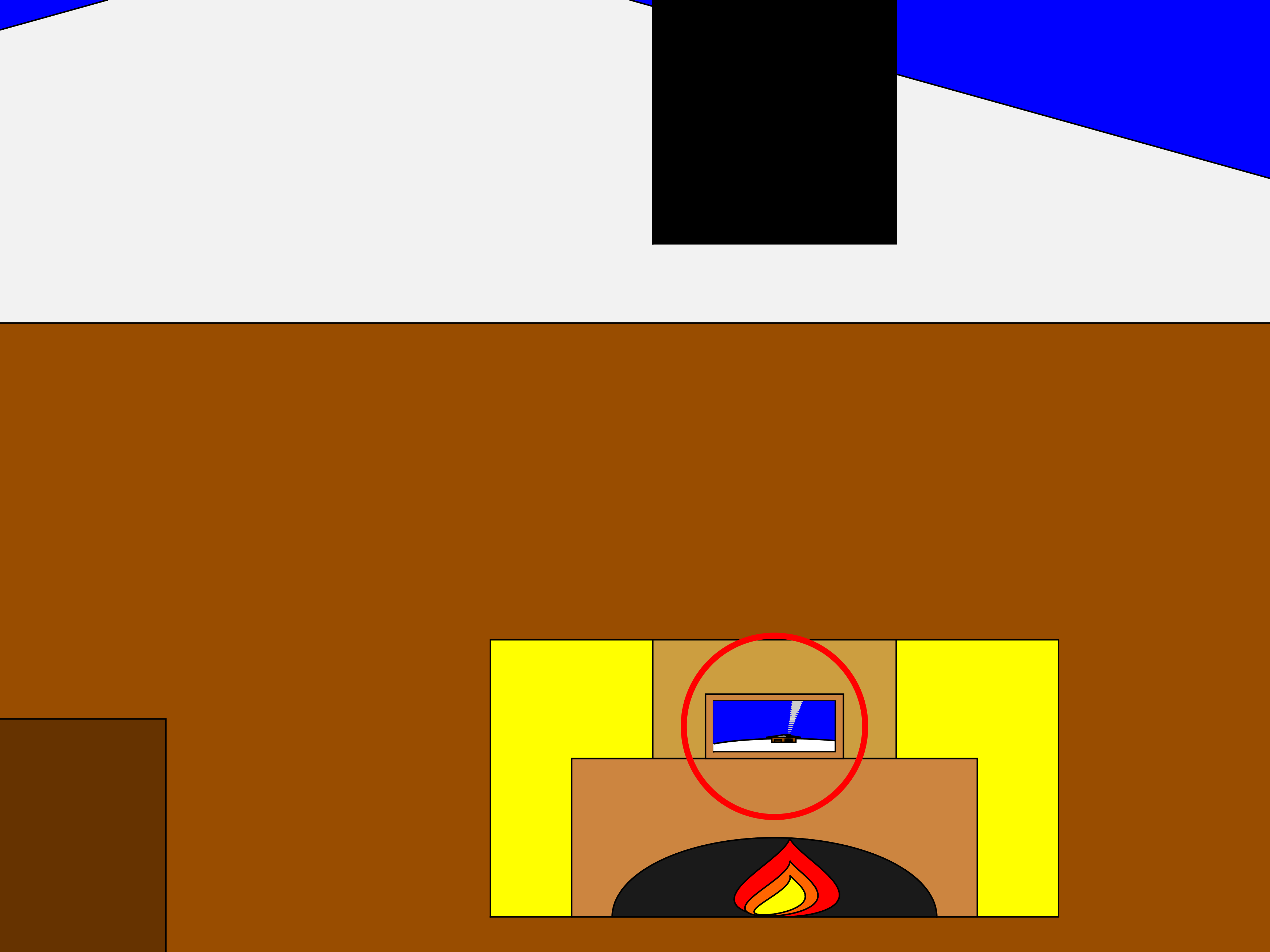
The implementation for this in 2-D is rather simple. Essentially, a second axes is used as the photograph. This is an efficient way of neatly updating the graphics while zooming in. The way this was implemented is explained in the following code snippet, which is a slight modification of the code in the entry:
m = 96; % Number of frames
% Axes limits for the first frame
xm = [xm1,xm2];
ym = [ym1,ym2];
% Axes limits for the last frame (photograph frame edges)
xf = [xf1,xf2];
yf = [yf1,yf2];
% Zoom-in vectors
x1 = linspace(xm(1),xf(1),m+1); % Axes left edge to left photo frame edge
x2 = linspace(xm(2),xf(2),m+1); % Axes right edge to right photo frame edge
y1 = linspace(ym(1),yf(1),m+1); % Axes bottom edge to bottom photo frame edge
y2 = linspace(ym(2),yf(2),m+1); % Axes top edge to top photo frame edge
if f==1
axis([x1(f),x2(f),y1(f),y2(f)]); % Set main axes limits
ax2 = copyobj(gca,gcf); % Create axes for the photo frame containing the first frame graphics objects
end
axis([x1(f+1),x2(f+1),y1(f+1),y2(f+1)]); % Zoom in main axes
lims = axis; % Main axes updated limits
pos = get(gca,'Position'); % Main axes position
% This keeps the relative position of the 2 axes constant:
pos = [pos(1)+diff([lims(1),xf(1)])/diff(lims(1:2))*pos(3),...
pos(2)+diff([lims(3),yf(1)])/diff(lims(3:4))*pos(4),...
diff(xf)/diff(lims(1:2))*pos(3),...
diff(yf)/diff(lims(3:4))*pos(4)];
ax2.Position = pos; % Adjust the relative position
Let's break down the code to explain the process:
- m is the total number of frames in the animation, i.e. 96 frames.
- xm & ym are the main axes limits for frame 1.
- xf & yf are the main axes limits for frame 96, corresponding to the photograph frame's edges.
- x1, x2, y1 & y2 are the zoom-in vectors, linearly spaced from the left, right, bottom & top main axes edges to the corresponding photograph edges. You have probably noticed that these contain m+1=97 points, which is 1 more than the total number of frames. This is done so that the first frame of the animation and the contents of the photograph frame are offset by a single timestep, so that there are no overlapping frames when the animation is looped, thus creating a perfect, seamless loop. That means that the first frame of the animation will contain the main axes zoomed-in by a single timestep, while the last frame of the animation (i.e. the zoomed-in photograph frame) will contain the most zoomed-out version of the graphics. This neatly wraps the animation, and displays the full zoomed-out view when the video stops playing.
- The photograph frame axes are created when f==1 (after setting the initial axes limits) by using the immensely useful copyobj function. This one-liner creates axes containing all graphics objects for the first frame.
- Zooming in on the main axes is then achieved by adjusting the limits using axis([x1(f+1),x2(f+1),y1(f+1),y2(f+1)]). The main axes current limits and position are then saved using the variables lims and pos respectively, in order to adjust the position of the photograph frame axes.
- While zooming in, it's important that the relative position of the 2 axes is kept constant. This is achieved by simply adjusting the position of the photograph frame axes at every frame, by calculating their relative ratios using the abovementioned formula. The first 2 arguments correspond to the (normalized) x and y positions of the lower left corner of the axes, while the third and fourth arguments correspond to the (normalized) width and height respectively. While this formula will work for any position of the main axes, it's a good idea to set the position as set(gca,'Position',[0 0 1 1]) for this contest, in order to take full advantage of the whole allocated window for the animation.
- Finally, note that the graphics are updated for the main axes only, and the above process is repeated for each frame until fully zooming into the photograph frame's axes.
Some of the most curious minds might wonder that while this is well and all with using the second axes to simulate the photograph, what happens to the photograph inside the photograph (and so on...)? Well, the beauty of this method is that you can repeat this as many times as necessary (just apply the formula using the current position and limits of the second axes to adjust the position of the third axes and so on). Given the speed of the animation and the very small size of the photograph inside the photograph, it would be very unlikely that you would need more than 3 axes, but the process is always good to know.
This is the final result:
I hope you found these tips useful and I'm looking forward to seeing many creative seamless loop animations in the contest.
MAThematical LABor
3%
MAth Theory Linear AlgeBra
12.5%
MATrix LABoratory
84%
MATthew LAst Breakthrough
0%
32 个投票
At School / university
64%
At work
30%
At home
3%
Elsewhere
3%
33 个投票
I am using Mathlab/simulink R2023b and PSIM2022.1.
I am trying to do co-simulación betwen simulink and PSIM of multiport controlled inverters. In Simulink, when I add the simcoupler block and double clik in it to set the path, that windows is opened, but when browse the path of PSIM schematic file and then clik APPLY, suddenly Simulink closes. Could somebody give some clue How to solve this issue.
NOTE: I tried as well the example of the tutorial of simcoupler module but the problem is the same.
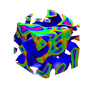
Here presented MATLAB code is designed to create a seamless loop animation that visualizes an isosurface derived from random data.
This entry, titled "The Scrambled Predator's Cube", builds upon my previous work and has been adapted to include dynamic elements.
In this explanation, I will break down the relatively short code, making it accessible whether you are a beginner in MATLAB or an experienced user. Let's go through the MATLAB code step by step to understand each line in detail.
Code Breakdown
d = rand(8,8,8);
Random Data Generation: This line creates a three-dimensional array d with dimensions 8×8×8 filled with random values. The rand function generates values uniformly distributed in the interval (0,1). This array serves as the input data for generating the isosurface.
iv = .5 + (f / 10000);
Isovalue Calculation: Here, the isovalue iv is computed based on the frame number f. The expression f / 10000 causes iv to increase very slowly as f increments. Starting from 0.50, this means that for every increment of f, iv changes slightly (specifically, by 0.0001). This gradual increase creates a smooth transition effect in the isosurface over time, making it look dynamic as the animation progresses.
h = patch(isosurface(d, iv), 'FaceColor', 'blue', 'EdgeColor', 'none');
Isosurface Creation: The isosurface function extracts a 3D surface from the data array d at the specified isovalue iv. The result is a patch object h that represents the isosurface in the 3D plot. The 'FaceColor', 'blue' argument sets the face color of the surface to blue, while 'EdgeColor', 'none' specifies that no edges should be drawn, giving the surface a solid appearance.
isonormals(d, h);
Surface Normals Calculation: This function calculates the normals at each vertex of the isosurface h, based on the data in d. Normals are vectors perpendicular to the surface at each point and are crucial for proper lighting calculations. By using isonormals, the appearance of depth and texture is enhanced, allowing the lighting to interact more realistically with the surface.
patch(isocaps(d, iv), 'FaceColor', 'interp', 'EdgeColor', 'none');
Isocaps Visualization: The isocaps function creates flat surfaces (caps) at the boundaries of the isosurface where the data values meet the isovalue iv. The resulting caps are then rendered as patches with 'FaceColor', 'interp', meaning the colors of the caps are interpolated based on the data values. The caps provide a more complete visual representation of the isosurface, improving its overall appearance.
colormap hsv;
Color Map Setup: This line sets the colormap of the current figure to HSV (Hue, Saturation, Value). The HSV colormap allows for a wide range of colors, which can enhance the visual appeal of the rendering by mapping different values in the data to different colors.
daspect([1, 1, 1]);
Aspect Ratio Setting: The daspect function sets the data aspect ratio of the plot to be equal in all three dimensions. This means that one unit in the x-direction is the same length as one unit in the y-direction and z-direction, ensuring that the visual representation of the 3D data is not distorted.
axis tight;
Tight Axis Setting: This command adjusts the limits of the axes so that they fit tightly around the data, removing any excess white space. It helps to focus the viewer's attention on the isosurface and related visual elements.
view(3);
3D View Configuration: The view(3) command sets the current view to a 3D perspective, allowing the viewer to see the structure of the isosurface from an angle that reveals its three-dimensional nature.
camlight right;
camlight left;
Lighting Effects: These commands add two light sources to the scene, positioned to the right and left of the view. The additional lighting enhances the shading and depth perception of the isosurface, making it appear more three-dimensional and visually appealing.
axis off;
Hide Axes: This command turns off the display of the axes in the plot. Removing the axes provides a cleaner visual representation, allowing the viewer to focus solely on the isosurface and its lighting effects without distraction from the grid lines or axis labels.
lighting phong;
Lighting Model: This line sets the lighting model to Phong. The Phong model is widely used in computer graphics as it provides smooth shading and realistic reflections. It calculates how light interacts with surfaces, enhancing the overall appearance by creating a more natural look.
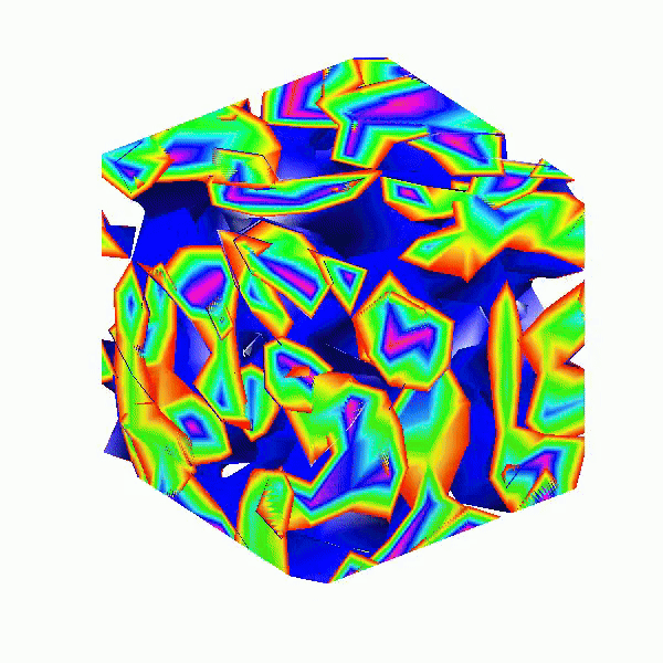
This code creates a visually dynamic and appealing representation of an isosurface derived from random data. The gradual change in the isovalue allows for smooth transitions, while the combination of lighting, colors, and shading contributes to a rich 3D visualization. Each component plays a vital role in rendering the final output, showcasing advanced techniques in data visualization using MATLAB.
I'd like to share some tips about the 2024 mini hack contest, specifically related to audio:
- First (and most important), credit your source: unless you are composing your own audio, I think it's important to give credit to the original sources. It is a little sad to see several contributions with an empty line:
'Cite your audio source here (if applicable):'
- A great place to get royalty-free and high-quality music and audio (among other media) is https://pixabay.com. Be sure to check it out! I used one of their audio clips in my submission EKG pulse
- The right music can enhance the overall experience of your animation. Sometimes getting the animation to match the music beat can be hard. I suggest you try the other way around: get your music/sound effects to match the animation rhythm with a little editing. A free audio editor with many capabilities (more than enough for this contest, I think) is https://www.audacityteam.org/
- Choose a 4-second audio clip with a consistent tempo and seamless loop points, ensuring it complements your animation's mood and loops smoothly over 12 seconds without abrupt changes.
I think that when the right music is paired with the right animation, it can create a more impactful experience.
Well, this is my first time to participate in such community competitions and guess what, I've gone for 4 submissions so far (Feels Great!!)
So I wanna share some tricks that I followed for my first submission named Happy Shaping' ( Go Check it out!!):
1. Dynamic Background Color Change:
- Technique: The background color of the figure window is gradually changed using sine and cosine functions.
- Reason: These trigonometric functions (sin and cos) create smooth, oscillating transitions over time, which gives a fluid effect to the background's color shift.
- Implementation:
Color = [0.1 + 0.5*abs(sin(f/10)), 0.1 + 0.5*abs(cos(f/15)), 0.9 -
0.5*abs(sin(f/20))];
- Benefit: This introduces a smooth, visually appealing animation effect.
2. Smooth Object Motion Using Sine and Cosine:
- Technique: The position and shape of objects are based on trigonometric functions.
- Reason: Using sin(t) and cos(t) ensures that the movement is circular or elliptical, creating continuous and natural motion in animations.
- Implementation (for object position):
x = 10 * cos(t * 2 * pi) * (1 + 0.5 * sin(t * pi));
y = 10 * sin(t * 2 * pi) * (1 + 0.5 * cos(t * pi));
- Benefit: Circular and smooth motions are pleasing and easily controlled by tweaking the frequency and phase of sine/cosine functions.
3. Polygon Shape Changing Over Time:
- Technique: The number of sides of the polygon (sides) changes dynamically based on t.
- Reason: It creates variation in shape, maintaining user interest as the shape transitions from a triangle to a hexagon.
- Implementation:
sides = 3 + round(3 * abs(sin(t)));
- Benefit: This provides dynamic shape transitions over time, keeping the animation non-static.
4. Use of the fill Function for Color-Filled Shapes:
- Technique: The fill function is used to draw a polygon with smoothly changing colors.
- Reason: Filling polygons with varying colors based on time (t) allows for continuous color transitions, adding more complexity to the animation.
- Implementation:
fill(xp, yp, c, 'EdgeColor', 'none');
- Benefit: Combining both color changes and shape changes enhances the visual impact.
5. Consistent Use of hold on and hold off:
- Technique: hold on allows multiple graphic objects to be drawn on the same axes without clearing previous objects.
- Reason: This is crucial for drawing multiple elements (like polygons, circles, and lines) on the same figure.
- Benefit: It helps manage and layer different graphical elements effectively within the same frame.
6. Use of rectangle for a Smooth Ball Motion:
- Technique: The ball's motion is defined by rectangle with a Curvature of [1, 1] to make it circular.
- Reason: Using the rectangle function simplifies the process of drawing a filled circle, and controlling its position and size is intuitive.
- Benefit: It provides a straightforward way to animate circular objects within the plot.
7. Animating the Connection Line:
- Technique: A white dashed line (w--) is drawn between the polygon and the moving ball to show a connection between these objects.
- Reason: This adds interactivity to the scene, as it gives the impression that the polygon and the ball are related or connected in some way.
- Implementation:
plot([x bx], [y by], 'w--', 'LineWidth', 2);
- Benefit: A dynamic element that adds depth and narrative to the animation, guiding the viewer’s attention.
8. Frame Synchronization with Time (f and t):
- Technique: The variable f is used as a frame number, while t = f / 24 creates a link between frame and time.
- Reason: Ensuring smooth and continuous transitions in the animation over time is critical, so f acts as the control for time-based changes in shape, color, and position.
- Benefit: This makes it easy to manage frame rates and time-based updates for the animation.
If you like them, please feel free to use them for free.
Try to install MATLAB2024a on Ubuntu24.04. In the image below, the button indicated by the green arrow is clickable, while the button indicated by the red arrow are unclickable, and input field where text cannot be entered, preventing the installation.

Do you use MATLAB Online for teaching? MATLAB Online lets students run MATLAB without having to install the software on the computer. All you need is a web browser and an internet connection.
I would love to hear comments and experiences of using MATLAB Online.
Let's say you have a chance to ask the MATLAB leadership team any question. What would you ask them?
If I go to a paint store, I can get foldout color charts/swatches for every brand of paint. I can make a selection and it will tell me the exact proportions of each of base color to add to a can of white paint. There doesn't seem to be any equivalent in MATLAB. The common word "swatch" doesn't even exist in the documentation. (?) One thinks pcolor() would be the way to go about this, but pcolor documentation is the most abstruse in all of the documentation. Thanks 1e+06 !
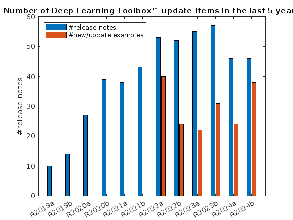
What is the side-effect of counting the number of Deep Learning Toolbox™ updates in the last 5 years? The industry has slowly stabilised and matured, so updates have slowed down in the last 1 year, and there has been no exponential growth.Is it correct to assume that? Let's see what you think!
releaseNumNames = "R"+string(2019:2024)+["a";"b"];
releaseNumNames = releaseNumNames(:);
numReleaseNotes = [10,14,27,39,38,43,53,52,55,57,46,46];
exampleNums = [nan,nan,nan,nan,nan,nan,40,24,22,31,24,38];
bar(releaseNumNames,[numReleaseNotes;exampleNums]')
legend(["#release notes","#new/update examples"],Location="northwest")
title("Number of Deep Learning Toolbox™ update items in the last 5 years")
ylabel("#release notes")
As pointed out in Doxygen comments in code generated with Simulink Embedded Coder - MATLAB Answers - MATLAB Central (mathworks.com), it would be nice that Embedded Coder has an option to generate Doxygen-style comments for signals of buses, i.e.:
/** @brief <Signal desciption here> **/
This would allow static analysis tools to parse the comments. Please add that feature!
How can I mechanically couple synchronous reluctance motor from simscape electrical electromechanical library and dc generator from specialized power system library
See the attached PDF for a higher resolution
Related blogs posts:
Hot off the heels of my High Performance Computing experience in the Czech republic, I've just booked my flights to Atlanta for this year's supercomputing conference at SC24.
Will any of you be there?
syms u v
atan2alt(v,u)
function Z = atan2alt(V,U)
% extension of atan2(V,U) into the complex plane
Z = -1i*log((U+1i*V)./sqrt(U.^2+V.^2));
% check for purely real input. if so, zero out the imaginary part.
realInputs = (imag(U) == 0) & (imag(V) == 0);
Z(realInputs) = real(Z(realInputs));
end
As I am editing this post, I see the expected symbolic display in the nice form as have grown to love. However, when I save the post, it does not display. (In fact, it shows up here in the discussions post.) This seems to be a new problem, as I have not seen that failure mode in the past.
You can see the problem in this Answer forum response of mine, where it did fail.
As far as I know, starting from MATLAB R2024b, the documentation is defaulted to be accessed online. However, the problem is that every time I open the official online documentation through my browser, it defaults or forcibly redirects to the documentation hosted site for my current geographic location, often with multiple pop-up reminders, which is very annoying!
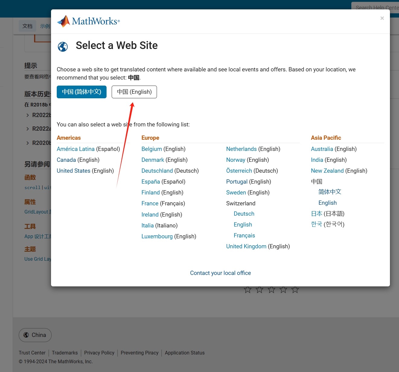
Suggestion: Could there be an option to set preferences linked to my personal account so that the documentation defaults to my chosen language preference without having to deal with “forced reminders” or “forced redirection” based on my geographic location? I prefer reading the English documentation, but the website automatically redirects me to the Chinese documentation due to my geolocation, which is quite frustrating!
----------------2024.12.13 update-----------------
Although the above issue was resolved by technical support, subsequent redirects are still causing severe delays...
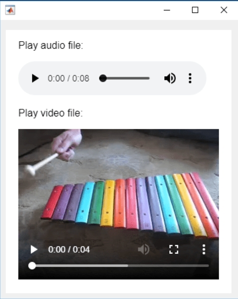
In the past two years, MATHWORKS has updated the image viewer and audio viewer, giving them a more modern interface with features like play, pause, fast forward, and some interactive tools that are more commonly found in typical third-party players. However, the video player has not seen any updates. For instance, the Video Viewer or vision.VideoPlayer could benefit from a more modern player interface. Perhaps I haven't found a suitable built-in player yet. It would be great if there were support for custom image processing and audio processing algorithms that could be played in a more modern interface in real time.
Additionally, I found it quite challenging to develop a modern video player from scratch in App Designer.(If there's a video component for that that would be great)
-----------------------------------------------------------------------------------------------------------------
BTW,the following picture shows the built-in function uihtml function showing a more modern playback interface with controls for play, pause and so on. But can not add real-time image processing algorithms within it.
您也可以从以下列表中选择网站:
美洲
- América Latina (Español)
- Canada (English)
- United States (English)
欧洲
- Belgium (English)
- Denmark (English)
- Deutschland (Deutsch)
- España (Español)
- Finland (English)
- France (Français)
- Ireland (English)
- Italia (Italiano)
- Luxembourg (English)
- Netherlands (English)
- Norway (English)
- Österreich (Deutsch)
- Portugal (English)
- Sweden (English)
- Switzerland
- United Kingdom(English)
亚太
- Australia (English)
- India (English)
- New Zealand (English)
- 中国
- 日本Japanese (日本語)
- 한국Korean (한국어)