搜索
Watch episodes 5-7 for the new stuff, but the whole series is really great.
I have one question.
Would it be possible to purchase Matlab for our company and incorporate the functions provided by this software into our in-house developed software to offer it to customers? Is this kind of action permitted under the license terms? I would appreciate advice from someone knowledgeable on this matter.
Just in two weeks, we already have 150+ entries! We are so impressed by your creative styles, artistic talents, and ingenious programming techniques.
Now, it’s time to announce the weekly winners!
Mini Hack Winners - Week 2
Seamless loop:
Nature & Animals:
Game:
Synchrony:
Remix of previous Mini Hack entries
Movie:
Congratulations to all winners! Each of you won your choice of a T-shirt, a hat, or a coffee mug. We will contact you after the contest ends.
In week 3, we’d love to see and award entries in the ‘holiday’ category.
Weekly Special Prizes
Thank you for sharing your tips & tricks with the community. You won limited-edition MATLAB Shorts.
We highly encourage everyone to share various types of content, such as tips and tricks for creating animations, background stories of your entry, or learnings you've gained from the contest.
Inspired by the suggestion of Mr. Chen Lin (MathWorks), I am writing this post with a humble and friendly intent to share some fascinating insights and knowledge about the Schwarzschild radius. My entry, which is related to this post, is named: 'Into the Abyss - Schwarzschild Radius (a time lapse)'.
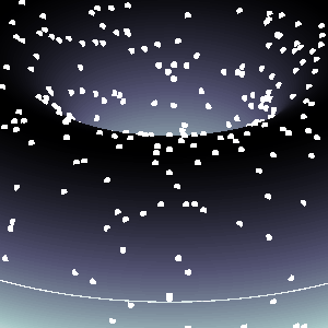
The Schwarzschild radius (or gravitational radius) defines the radius of the event horizon of a black hole, which is the boundary beyond which nothing, not even light, can escape the gravitational pull of the black hole. This concept comes from the Schwarzschild solution to Einstein’s field equations in general relativity. Black holes are regions of spacetime where gravitational collapse has caused matter to be concentrated within such a small volume that the escape velocity exceeds the speed of light.
This is a rudimentary scientific post, as the matter of Schwarzschild radius - it's true meaning and function, is a much, much, much-more complex "thing" (not known to us entierly, by the third degre of epistemological explanation(s)).
And, very important is to mention: I am NOT an expert - by any means, on this topic, just a very curious guy, in almost anything, that has to do with science.
Schwarzschild Radius (Gravitational Radius)
The Schwarzschild radius (Rₛ) is the critical radius at which an object of mass  must be compressed to form a black hole, specifically, a non-rotating, uncharged black hole, known as a Schwarzschild black hole. The Schwarzschild radius
  is given by the formula:
 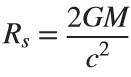 .
.
is given by the formula: . Where: 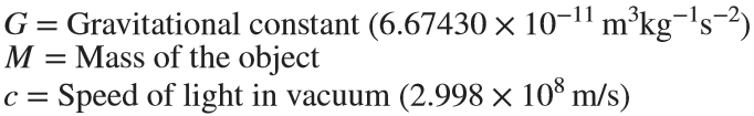 .
.
. Key Characteristics are, that for any mass, if that mass is compressed within a sphere with radius equal to  , the gravitational field is so strong that not even light can escape, thus forming a black hole. The Schwarzschild radius is proportional to the mass. Larger masses have larger Schwarzschild radii.
, the gravitational field is so strong that not even light can escape, thus forming a black hole. The Schwarzschild radius is proportional to the mass. Larger masses have larger Schwarzschild radii.Example:
For the Sun  :
: 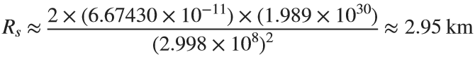 .
.
: .So, if the Sun were compressed into a sphere with a radius of ~3 km, it would become a black hole!
Stellar-mass Black Holes form from the collapse of massive stars (roughly 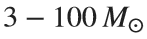 ). Their Schwarzschild radius ranges from a few kilometers to tens of kilometers.
). Their Schwarzschild radius ranges from a few kilometers to tens of kilometers. Supermassive Black Holes found at the centers of galaxies, such as Sagittarius A in the Milky Way ( ), their Schwarzschild radii span from a few million to billions of kilometers!
), their Schwarzschild radii span from a few million to billions of kilometers! Primordial or Micro Black Holes, are the hypothetical small black holes with masses much smaller than stellar masses, where the Schwarzschild radius could be extremely tiny.
A black hole, in general, is a solution to Einstein’s general theory of relativity where spacetime is curved to such an extent that nothing within a certain region, called the event horizon, can escape.
Types of Black Holes:
1. Schwarzschild (Non-rotating, Uncharged):
- This is the simplest type of black hole, described by the Schwarzschild solution.
- Its key feature is the singularity at the center, where the curvature of spacetime becomes infinite.
- No charge, no angular momentum (spin), and spherical symmetry.
2. Kerr (Rotating):
- Describes rotating black holes.
- Involves an additional parameter called angular momentum.
- Has an event horizon and an inner boundary, known as the ergosphere, where spacetime is dragged around by the black hole's rotation.
3. Reissner–Nordström (Charged, Non-rotating):
- A black hole with electric charge.
- A charged black hole has two event horizons (inner and outer) and a central singularity.
4. Kerr–Newman (Rotating and Charged):
- The most general solution, describing a black hole that has both charge and angular momentum.
Relationship Between Schwarzschild Radius and Black Holes
Formation of Black Holes: When a massive star exhausts its nuclear fuel, gravitational collapse can compress the core beyond the Schwarzschild radius, creating a black hole.
Event Horizon: The Schwarzschild radius marks the event horizon for a non-rotating black hole. This is the boundary beyond which no information or matter can escape the black hole.
Curvature of Spacetime: At distances closer than the Schwarzschild radius, spacetime curvature becomes so extreme that all paths, even those of light, are bent towards the black hole’s singularity.
BTW, the term singularity, scientificaly 😊, means that: we do not have a clue what is really happening right there...
Detailed Properties of Black Holes:
a. Singularity:
At the center of a black hole, within the Schwarzschild radius, lies the singularity, a point (or ring in the case of rotating black holes) where gravitational forces compress matter to infinite density and spacetime curvature becomes infinite. General relativity breaks down at the singularity, and a quantum theory of gravity is required for a complete understanding.
b. Event Horizon:
The event horizon is not a physical surface but a boundary where the escape velocity equals the speed of light. For an outside observer, objects falling into a black hole appear to slow down and fade away near the event horizon due to gravitational time dilation, a prediction of general relativity. From the perspective of the infalling object, however, it crosses the event horizon in finite time without noticing anything special at the moment of crossing.
c. Hawking Radiation: (In the post, I told that there is no radiation - to make it simple, although, there is a relatively newly-found (theoretically) radiation. Truth to be said, some physicists are still chalenging this notion, in some of it's parts...)
Quantum mechanical effects near the event horizon predict that black holes can emit radiation (Hawking radiation), a process through which black holes can lose mass and, over very long timescales, potentially evaporate completely. This process has a temperature inversely proportional to the black hole's mass, making large black holes emit extremely weak radiation. (Very trivialy speaking: the concept supposes that an anti-particle is drawn from the vakum and is anihilated with the black's hole matter (particle), and in the process, the black hole looses mass gradually and proportionally to the released energy - very slowly(!)).
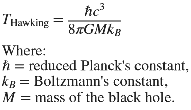
This radiation is significant only for small black holes.
Gravitational Time Dilation (here, as well, things become 'super-weird'...)
Near the Schwarzschild radius, the intense gravitational field leads to time dilation. For an external observer far from the black hole, time appears to slow down for an object moving toward the event horizon. As it approaches the Schwarzschild radius, time dilation becomes so extreme that the object appears frozen in time at the horizon.
The time dilation factor is given by: 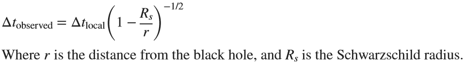
Eg. Approaching the Schwarzschild radius and theoretically remaining just outside of it for a few hours would correspond to the passage of approximately several decades on Earth due to relativistic time dilation.
Using relativistic equations, it's estimated that near the event horizon 2 hours (120 minutes) near the black hole Sagittarius A* (as already mentioned ~ 4 million  ) - in the center of our galaxy Milky Way, could correspond to 83 years passing on Earth! However, this varies based on the precise distance from the event horizon (give or take, a decade 😬).
) - in the center of our galaxy Milky Way, could correspond to 83 years passing on Earth! However, this varies based on the precise distance from the event horizon (give or take, a decade 😬).Information Paradox (definte answer on this question, 'hold's the keys of the universe' 😊, maybe...)
The black hole information paradox arises from the seeming contradiction between general relativity and quantum mechanics.
According to quantum mechanics, information cannot be destroyed, yet anything falling into a black hole seems to be lost beyond the event horizon. Hawking radiation, which allows a black hole to evaporate, does not appear to carry information about the matter that fell into the black hole, leading to ongoing debates and research into how information is preserved in the context of black holes, or not...!
Schwarzschild Radius is the key parameter defining the size of the event horizon of a non-rotating black hole. Black Holes are regions where the Schwarzschild radius constrains all physical phenomena due to extreme gravitational forces, forming event horizons and singularities. The interaction between general relativity and quantum mechanics in the context of black holes (e.g., Hawking radiation and the information paradox) remains one of the most intriguing areas in modern theoretical physics.
For detailed and further reading: https://www.sciencedirect.com/topics/physics-and-astronomy/hawking-radiation.
I hope you will find this post, and information provided, interesting.
This year's MATLAB Shorts Mini Hack contest has kicked off, and there are already lots of interesting entries. The contest features creating a 96-frame, 4-second animation, which is looped 3 times to compose a 12-second short movie. There is an option to add audio to enhance the animation, and it's restricted to a an upper limit of 2,000 characters to promote efficient coding.
Many of the contestants have already realized the potential for creating a seamless loop, which provides a smooth transition and avoids any discontinuities when the animation is repeated. There are several ways to achieve this. An efficient method for example is utilizing sinusoidal functions, which are periodic, meaning that they repeat themselves over time:
An intuitive example of a seamless loop is @Edgar Guevara's EKG pulse entry, which features an electrocardiogram signal on an oscilloscope. The animation is perfectly matched by the audio, as explained in their post.
Another, rather sophisticated approach is featured in @Tim's Moonrun animation in last year's contest. This seamless loop is achieved by cleverly manipulating the camera position and target over a periodic spatial domain, producing this stunning result:
This essentially tells us that for a seamless loop in the spatial domain, the first frame must match the last frame (with a single timestep difference to be more precise, more on that later). But surely this cannot be achieved by zooming in, unless you are simulating a fractal. Well, there are always workarounds.
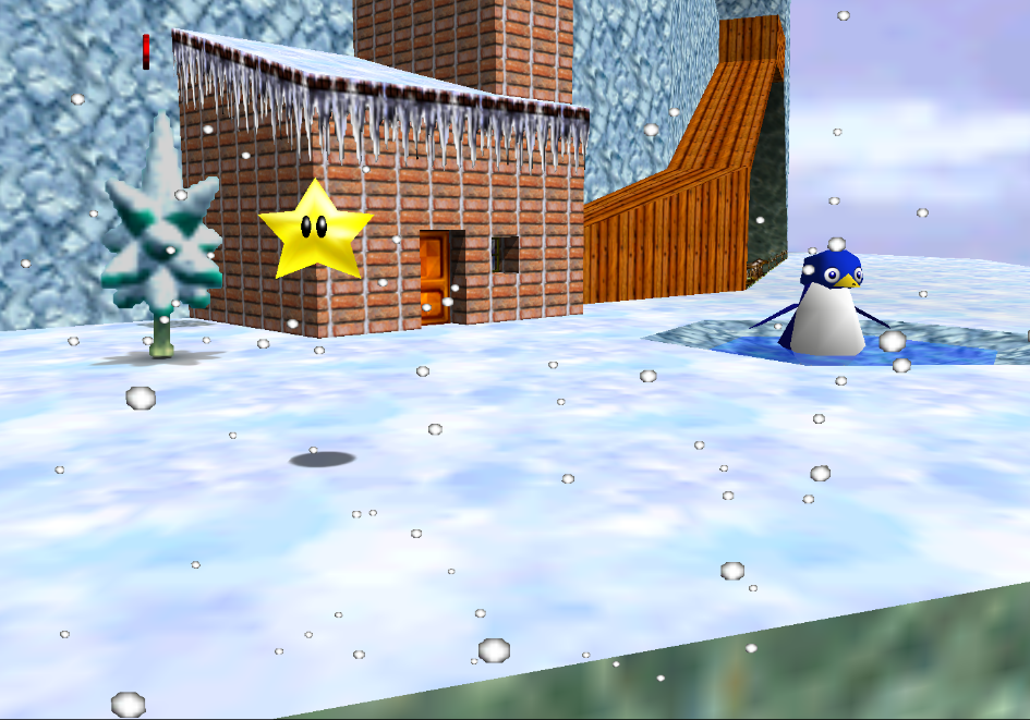
One way to achieve this is by zooming into a section that contains the first frame of the animation. This is featured in my Winter Loop entry. This is a remix of @Oliver Jaros's Winter entry, which was selected as a one of the weekly winners in the nature & space category for Week 1. The code was modified to lower the character count, but all credits for the original idea and graphics go to them. I also drew inspiration from one of my favourite games of all time, Super Mario 64. Oliver's animation reminded me of the Cool, Cool Mountain level of the game. In the game, you can enter various levels by jumping into paintings serving as portals.
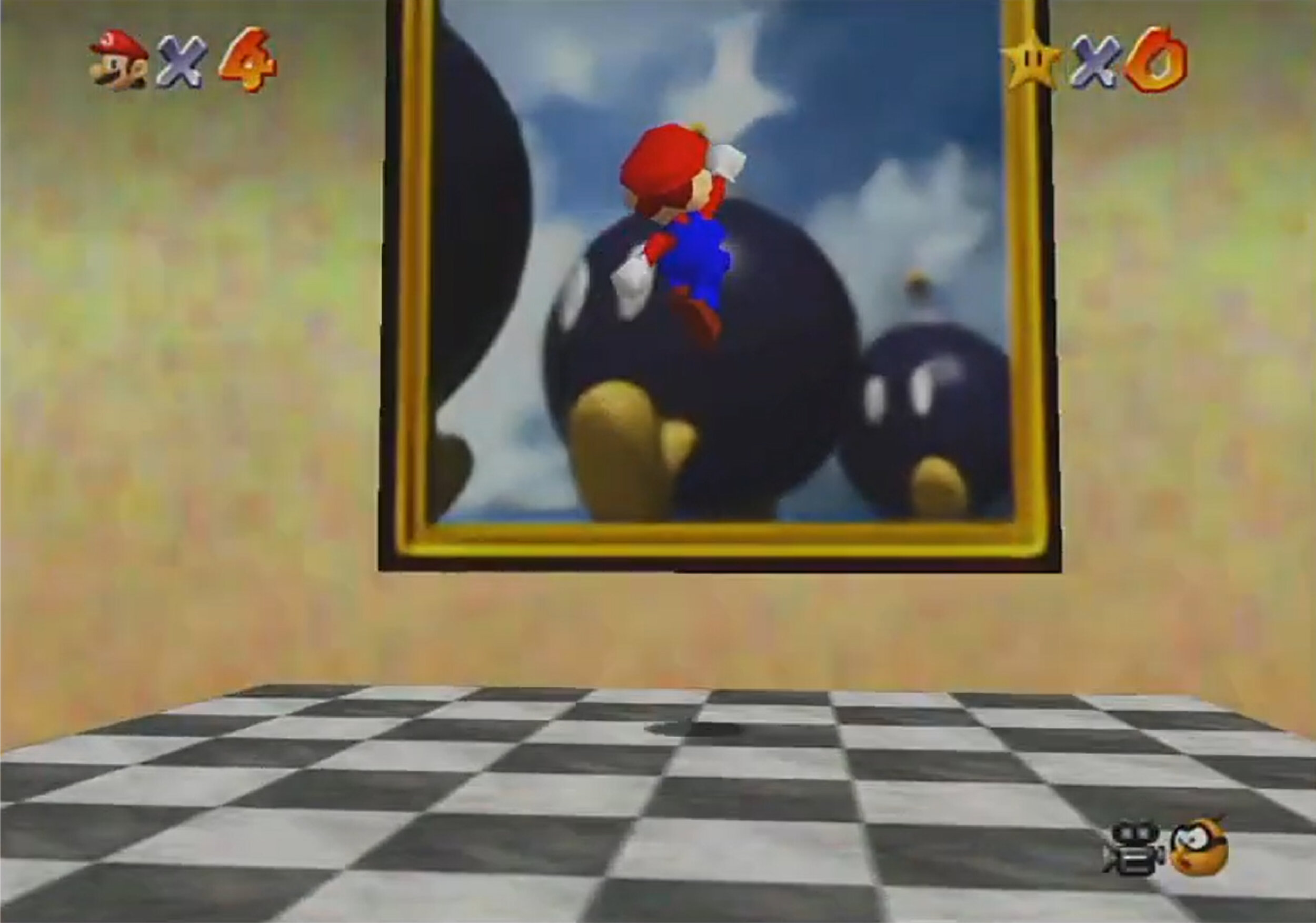
This inspired the idea of zooming into a rectangular photograph frame containing the first frame of the animation to facilitate restarting the loop. One could argue that it would probably take a crazy person to have a photo of their house framed inside their own house. Well, in this economy and with the current house prices, I don't think this scenario is too far-fetched:
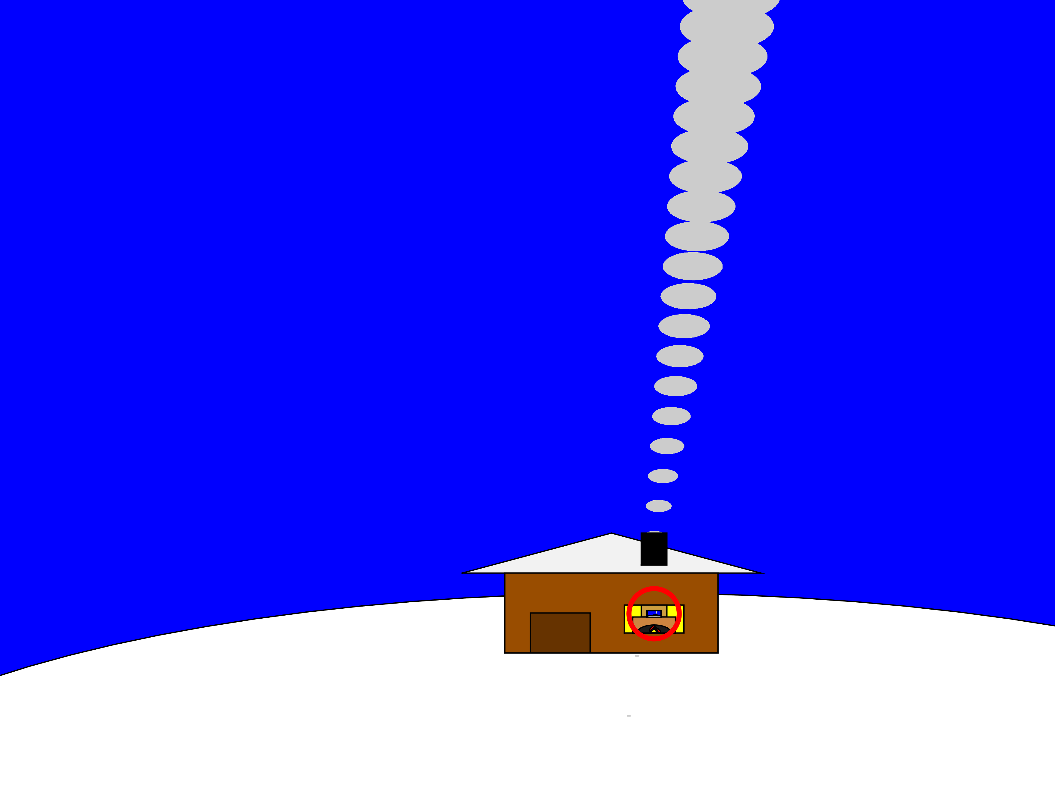
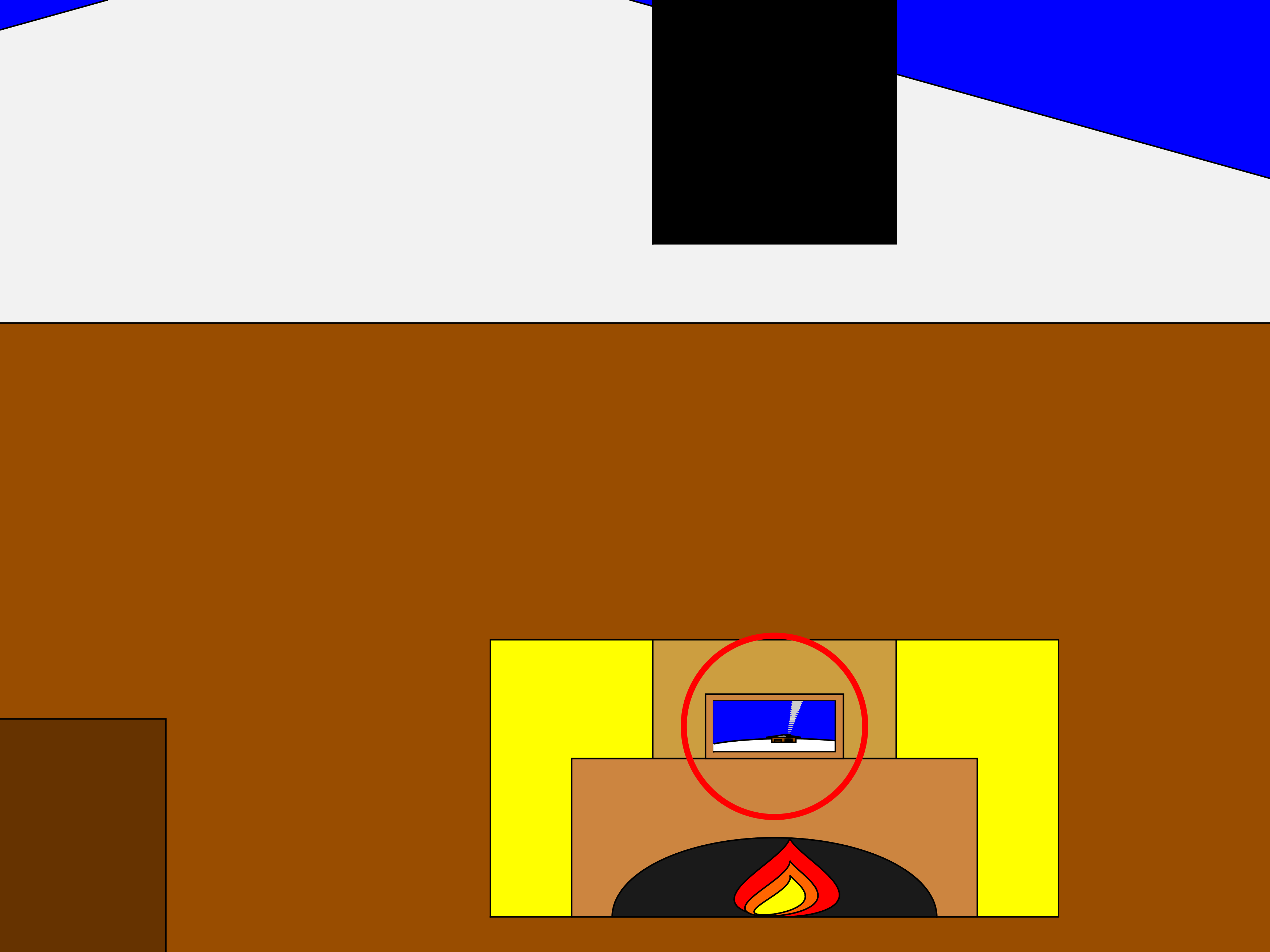
The implementation for this in 2-D is rather simple. Essentially, a second axes is used as the photograph. This is an efficient way of neatly updating the graphics while zooming in. The way this was implemented is explained in the following code snippet, which is a slight modification of the code in the entry:
m = 96; % Number of frames
% Axes limits for the first frame
xm = [xm1,xm2];
ym = [ym1,ym2];
% Axes limits for the last frame (photograph frame edges)
xf = [xf1,xf2];
yf = [yf1,yf2];
% Zoom-in vectors
x1 = linspace(xm(1),xf(1),m+1); % Axes left edge to left photo frame edge
x2 = linspace(xm(2),xf(2),m+1); % Axes right edge to right photo frame edge
y1 = linspace(ym(1),yf(1),m+1); % Axes bottom edge to bottom photo frame edge
y2 = linspace(ym(2),yf(2),m+1); % Axes top edge to top photo frame edge
if f==1
axis([x1(f),x2(f),y1(f),y2(f)]); % Set main axes limits
ax2 = copyobj(gca,gcf); % Create axes for the photo frame containing the first frame graphics objects
end
axis([x1(f+1),x2(f+1),y1(f+1),y2(f+1)]); % Zoom in main axes
lims = axis; % Main axes updated limits
pos = get(gca,'Position'); % Main axes position
% This keeps the relative position of the 2 axes constant:
pos = [pos(1)+diff([lims(1),xf(1)])/diff(lims(1:2))*pos(3),...
pos(2)+diff([lims(3),yf(1)])/diff(lims(3:4))*pos(4),...
diff(xf)/diff(lims(1:2))*pos(3),...
diff(yf)/diff(lims(3:4))*pos(4)];
ax2.Position = pos; % Adjust the relative position
Let's break down the code to explain the process:
- m is the total number of frames in the animation, i.e. 96 frames.
- xm & ym are the main axes limits for frame 1.
- xf & yf are the main axes limits for frame 96, corresponding to the photograph frame's edges.
- x1, x2, y1 & y2 are the zoom-in vectors, linearly spaced from the left, right, bottom & top main axes edges to the corresponding photograph edges. You have probably noticed that these contain m+1=97 points, which is 1 more than the total number of frames. This is done so that the first frame of the animation and the contents of the photograph frame are offset by a single timestep, so that there are no overlapping frames when the animation is looped, thus creating a perfect, seamless loop. That means that the first frame of the animation will contain the main axes zoomed-in by a single timestep, while the last frame of the animation (i.e. the zoomed-in photograph frame) will contain the most zoomed-out version of the graphics. This neatly wraps the animation, and displays the full zoomed-out view when the video stops playing.
- The photograph frame axes are created when f==1 (after setting the initial axes limits) by using the immensely useful copyobj function. This one-liner creates axes containing all graphics objects for the first frame.
- Zooming in on the main axes is then achieved by adjusting the limits using axis([x1(f+1),x2(f+1),y1(f+1),y2(f+1)]). The main axes current limits and position are then saved using the variables lims and pos respectively, in order to adjust the position of the photograph frame axes.
- While zooming in, it's important that the relative position of the 2 axes is kept constant. This is achieved by simply adjusting the position of the photograph frame axes at every frame, by calculating their relative ratios using the abovementioned formula. The first 2 arguments correspond to the (normalized) x and y positions of the lower left corner of the axes, while the third and fourth arguments correspond to the (normalized) width and height respectively. While this formula will work for any position of the main axes, it's a good idea to set the position as set(gca,'Position',[0 0 1 1]) for this contest, in order to take full advantage of the whole allocated window for the animation.
- Finally, note that the graphics are updated for the main axes only, and the above process is repeated for each frame until fully zooming into the photograph frame's axes.
Some of the most curious minds might wonder that while this is well and all with using the second axes to simulate the photograph, what happens to the photograph inside the photograph (and so on...)? Well, the beauty of this method is that you can repeat this as many times as necessary (just apply the formula using the current position and limits of the second axes to adjust the position of the third axes and so on). Given the speed of the animation and the very small size of the photograph inside the photograph, it would be very unlikely that you would need more than 3 axes, but the process is always good to know.
This is the final result:
I hope you found these tips useful and I'm looking forward to seeing many creative seamless loop animations in the contest.
MAThematical LABor
3%
MAth Theory Linear AlgeBra
12.5%
MATrix LABoratory
84%
MATthew LAst Breakthrough
0%
32 个投票
At School / university
64%
At work
30%
At home
3%
Elsewhere
3%
33 个投票
I am using Mathlab/simulink R2023b and PSIM2022.1.
I am trying to do co-simulación betwen simulink and PSIM of multiport controlled inverters. In Simulink, when I add the simcoupler block and double clik in it to set the path, that windows is opened, but when browse the path of PSIM schematic file and then clik APPLY, suddenly Simulink closes. Could somebody give some clue How to solve this issue.
NOTE: I tried as well the example of the tutorial of simcoupler module but the problem is the same.
Welcome to the launch of our new blog area, Semiconductor Design and Verification! The mission is to empower engineers and designers in the semiconductor industry by streamlining architectural exploration, optimizing the post-processing of simulations, and enabling early verification with MATLAB and Simulink.
Meet Our Authors
We are thrilled to have two esteemed authors:
@Ganesh Rathinavel and @Cristian Macario Macario have both made significant contributions to the advancement of Analog/Mixed-Signal design and the broader communications, electronics, and semiconductor industries. With impressive engineering backgrounds and extensive experience at leading companies such as IMEC, STMicroelectronics, NXP Semiconductors, LSI Corporation, and ARM, they bring a wealth of knowledge and expertise to our blog. Their work is focused on enhancing MathWorks' tools to better align with industry needs.
What to Expect
The blog will cover a wide range of topics aimed at professionals in the semiconductor field, providing insights and strategies to enhance your design and verification processes. Whether you're looking to streamline your current workflows or explore cutting-edge methodologies, our blog is your go-to resource.
Call to Action
We invite all professionals and enthusiasts in the semiconductor industry to follow our blog posts. Stay updated with the latest trends and insights by subscribing to our blog.

Don’t miss the first post: Accelerating Mixed-Signal Design with Early Behavioral Models, where they explore how early behavioral modeling can accelerate mixed-signal design and enhance system efficiency.
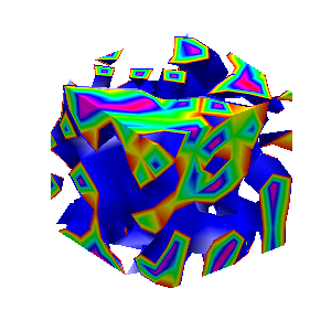
Here presented MATLAB code is designed to create a seamless loop animation that visualizes an isosurface derived from random data.
This entry, titled "The Scrambled Predator's Cube", builds upon my previous work and has been adapted to include dynamic elements.
In this explanation, I will break down the relatively short code, making it accessible whether you are a beginner in MATLAB or an experienced user. Let's go through the MATLAB code step by step to understand each line in detail.
Code Breakdown
d = rand(8,8,8);
Random Data Generation: This line creates a three-dimensional array d with dimensions 8×8×8 filled with random values. The rand function generates values uniformly distributed in the interval (0,1). This array serves as the input data for generating the isosurface.
iv = .5 + (f / 10000);
Isovalue Calculation: Here, the isovalue iv is computed based on the frame number f. The expression f / 10000 causes iv to increase very slowly as f increments. Starting from 0.50, this means that for every increment of f, iv changes slightly (specifically, by 0.0001). This gradual increase creates a smooth transition effect in the isosurface over time, making it look dynamic as the animation progresses.
h = patch(isosurface(d, iv), 'FaceColor', 'blue', 'EdgeColor', 'none');
Isosurface Creation: The isosurface function extracts a 3D surface from the data array d at the specified isovalue iv. The result is a patch object h that represents the isosurface in the 3D plot. The 'FaceColor', 'blue' argument sets the face color of the surface to blue, while 'EdgeColor', 'none' specifies that no edges should be drawn, giving the surface a solid appearance.
isonormals(d, h);
Surface Normals Calculation: This function calculates the normals at each vertex of the isosurface h, based on the data in d. Normals are vectors perpendicular to the surface at each point and are crucial for proper lighting calculations. By using isonormals, the appearance of depth and texture is enhanced, allowing the lighting to interact more realistically with the surface.
patch(isocaps(d, iv), 'FaceColor', 'interp', 'EdgeColor', 'none');
Isocaps Visualization: The isocaps function creates flat surfaces (caps) at the boundaries of the isosurface where the data values meet the isovalue iv. The resulting caps are then rendered as patches with 'FaceColor', 'interp', meaning the colors of the caps are interpolated based on the data values. The caps provide a more complete visual representation of the isosurface, improving its overall appearance.
colormap hsv;
Color Map Setup: This line sets the colormap of the current figure to HSV (Hue, Saturation, Value). The HSV colormap allows for a wide range of colors, which can enhance the visual appeal of the rendering by mapping different values in the data to different colors.
daspect([1, 1, 1]);
Aspect Ratio Setting: The daspect function sets the data aspect ratio of the plot to be equal in all three dimensions. This means that one unit in the x-direction is the same length as one unit in the y-direction and z-direction, ensuring that the visual representation of the 3D data is not distorted.
axis tight;
Tight Axis Setting: This command adjusts the limits of the axes so that they fit tightly around the data, removing any excess white space. It helps to focus the viewer's attention on the isosurface and related visual elements.
view(3);
3D View Configuration: The view(3) command sets the current view to a 3D perspective, allowing the viewer to see the structure of the isosurface from an angle that reveals its three-dimensional nature.
camlight right;
camlight left;
Lighting Effects: These commands add two light sources to the scene, positioned to the right and left of the view. The additional lighting enhances the shading and depth perception of the isosurface, making it appear more three-dimensional and visually appealing.
axis off;
Hide Axes: This command turns off the display of the axes in the plot. Removing the axes provides a cleaner visual representation, allowing the viewer to focus solely on the isosurface and its lighting effects without distraction from the grid lines or axis labels.
lighting phong;
Lighting Model: This line sets the lighting model to Phong. The Phong model is widely used in computer graphics as it provides smooth shading and realistic reflections. It calculates how light interacts with surfaces, enhancing the overall appearance by creating a more natural look.
This code creates a visually dynamic and appealing representation of an isosurface derived from random data. The gradual change in the isovalue allows for smooth transitions, while the combination of lighting, colors, and shading contributes to a rich 3D visualization. Each component plays a vital role in rendering the final output, showcasing advanced techniques in data visualization using MATLAB.
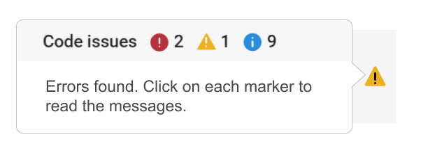
We are happy to announce the addition of a new code analyzing feature to the AI Chat Playground. This new feature allows you to identify issues with your code making it easier to troubleshoot.
How does it work?
Just click the ANALYZE button in the toolbar of the code editor. Your code is sent to MATLAB running on a server which returns any warnings or errors, each of which are associated to a line of code on the right side of the editor window. Hover over each line marker to view the message.
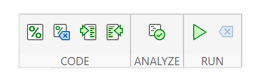
Give it a try and share your feedback here. We will be adding this new capability to other community areas in the future so your feedback is appreciated.
Thank you,
David
There are so many incredible entries created in week 1. Now, it’s time to announce the weekly winners in various categories!
Nature & Space:
Seamless Loop:
Abstract:
Remix of previous Mini Hack entries:
Early Discovery
Holiday:
Congratulations to all winners! Each of you won your choice of a T-shirt, a hat, or a coffee mug. We will contact you after the contest ends.
In week 2, we’d love to see and award more entries in the ‘Seamless Loop’ category. We can't wait to see your creativity shine!
Tips for Week 2:
1.Use AI for assistance
The code from the Mini Hack entries can be challenging, even for experienced MATLAB users. Utilize AI tools for MATLAB to help you understand the code and modify the code. Here is an example of a remix assisted by AI. @Hans Scharler used MATLAB GPT to get an explanation of the code and then prompted it to ‘change the background to a starry night with the moon.’
2. Share your thoughts
Share your tips & tricks, experience of using AI, or learnings with the community. Post your knowledge in the Discussions' general channel (be sure to add the tag 'contest2024') to earn opportunities to win the coveted MATLAB Shorts.
3. Ensure Thumbnails Are Displayed:
You might have noticed that some entries on the leaderboard lack a thumbnail image. To fix this, ensure you include ‘drawframe(1)’ in your code.
I'd like to share some tips about the 2024 mini hack contest, specifically related to audio:
- First (and most important), credit your source: unless you are composing your own audio, I think it's important to give credit to the original sources. It is a little sad to see several contributions with an empty line:
'Cite your audio source here (if applicable):'
- A great place to get royalty-free and high-quality music and audio (among other media) is https://pixabay.com. Be sure to check it out! I used one of their audio clips in my submission EKG pulse
- The right music can enhance the overall experience of your animation. Sometimes getting the animation to match the music beat can be hard. I suggest you try the other way around: get your music/sound effects to match the animation rhythm with a little editing. A free audio editor with many capabilities (more than enough for this contest, I think) is https://www.audacityteam.org/
- Choose a 4-second audio clip with a consistent tempo and seamless loop points, ensuring it complements your animation's mood and loops smoothly over 12 seconds without abrupt changes.
I think that when the right music is paired with the right animation, it can create a more impactful experience.
Well, this is my first time to participate in such community competitions and guess what, I've gone for 4 submissions so far (Feels Great!!)
So I wanna share some tricks that I followed for my first submission named Happy Shaping' ( Go Check it out!!):
1. Dynamic Background Color Change:
- Technique: The background color of the figure window is gradually changed using sine and cosine functions.
- Reason: These trigonometric functions (sin and cos) create smooth, oscillating transitions over time, which gives a fluid effect to the background's color shift.
- Implementation:
Color = [0.1 + 0.5*abs(sin(f/10)), 0.1 + 0.5*abs(cos(f/15)), 0.9 -
0.5*abs(sin(f/20))];
- Benefit: This introduces a smooth, visually appealing animation effect.
2. Smooth Object Motion Using Sine and Cosine:
- Technique: The position and shape of objects are based on trigonometric functions.
- Reason: Using sin(t) and cos(t) ensures that the movement is circular or elliptical, creating continuous and natural motion in animations.
- Implementation (for object position):
x = 10 * cos(t * 2 * pi) * (1 + 0.5 * sin(t * pi));
y = 10 * sin(t * 2 * pi) * (1 + 0.5 * cos(t * pi));
- Benefit: Circular and smooth motions are pleasing and easily controlled by tweaking the frequency and phase of sine/cosine functions.
3. Polygon Shape Changing Over Time:
- Technique: The number of sides of the polygon (sides) changes dynamically based on t.
- Reason: It creates variation in shape, maintaining user interest as the shape transitions from a triangle to a hexagon.
- Implementation:
sides = 3 + round(3 * abs(sin(t)));
- Benefit: This provides dynamic shape transitions over time, keeping the animation non-static.
4. Use of the fill Function for Color-Filled Shapes:
- Technique: The fill function is used to draw a polygon with smoothly changing colors.
- Reason: Filling polygons with varying colors based on time (t) allows for continuous color transitions, adding more complexity to the animation.
- Implementation:
fill(xp, yp, c, 'EdgeColor', 'none');
- Benefit: Combining both color changes and shape changes enhances the visual impact.
5. Consistent Use of hold on and hold off:
- Technique: hold on allows multiple graphic objects to be drawn on the same axes without clearing previous objects.
- Reason: This is crucial for drawing multiple elements (like polygons, circles, and lines) on the same figure.
- Benefit: It helps manage and layer different graphical elements effectively within the same frame.
6. Use of rectangle for a Smooth Ball Motion:
- Technique: The ball's motion is defined by rectangle with a Curvature of [1, 1] to make it circular.
- Reason: Using the rectangle function simplifies the process of drawing a filled circle, and controlling its position and size is intuitive.
- Benefit: It provides a straightforward way to animate circular objects within the plot.
7. Animating the Connection Line:
- Technique: A white dashed line (w--) is drawn between the polygon and the moving ball to show a connection between these objects.
- Reason: This adds interactivity to the scene, as it gives the impression that the polygon and the ball are related or connected in some way.
- Implementation:
plot([x bx], [y by], 'w--', 'LineWidth', 2);
- Benefit: A dynamic element that adds depth and narrative to the animation, guiding the viewer’s attention.
8. Frame Synchronization with Time (f and t):
- Technique: The variable f is used as a frame number, while t = f / 24 creates a link between frame and time.
- Reason: Ensuring smooth and continuous transitions in the animation over time is critical, so f acts as the control for time-based changes in shape, color, and position.
- Benefit: This makes it easy to manage frame rates and time-based updates for the animation.
Over the past week, we have seen many creative and compelling short movies! Now, let the voting begin! Cast your votes for the short movies you love. Authors, share your creations with friends, classmates, and colleagues. Let's showcase the beauty of mathematics to the world!
We know that one of the key goals for joining the Mini Hack contest is to LEARN! To celebrate knowledge sharing, we have special prizes—limited-edition MATLAB Shorts—up for grabs!
These exclusive prizes can only be earned through the MATLAB Shorts Mini Hack contest. Interested? Share your knowledge in the Discussions' general channel (be sure to add the tag 'contest2024') to earn opportunities to win the coveted MATLAB Shorts. You can share various types of content, such as tips and tricks for creating animations, background stories of your entry, or learnings you've gained from the contest. We will select different types of winners each week.

We also have an exciting feature announcement: you can now experiment with code in MATLAB Online. Simply click the 'Open in MATLAB Online' button above the movie preview section. Even better! ‘Open in MATLAB Online’ is also available in previous Mini Hack contests!

We look forward to seeing more amazing short movies in Week 2!
If you like them, please feel free to use them for free.
Try to install MATLAB2024a on Ubuntu24.04. In the image below, the button indicated by the green arrow is clickable, while the button indicated by the red arrow are unclickable, and input field where text cannot be entered, preventing the installation.

Do you use MATLAB Online for teaching? MATLAB Online lets students run MATLAB without having to install the software on the computer. All you need is a web browser and an internet connection.
I would love to hear comments and experiences of using MATLAB Online.
Let's say you have a chance to ask the MATLAB leadership team any question. What would you ask them?
We are thrilled to announce that every community member now has the ability to create a poll in Discussions, allowing you to gather votes and opinions from the community.
How to create a poll:
You can find the ‘Create a Poll’ link just below the text box (see screenshot below). Please note that the default type of content is a ‘Discussion’. To start a poll, simply click the link.

Creating a poll is straightforward. You can add up to 6 choices for your poll and set the duration from 1 to 6 weeks.

Where to find the poll
Polls created by community members will appear only in the channel where they are created and the landing page of Discussions area. Discussions moderators have the privilege to feature/broadcast the poll across Answers, File Exchange, and Cody.
Thoughts?
We can’t wait to see what interesting polls our community will create. Meanwhile, if you have any questions or suggestions, feel free to leave a comment.