搜索
📢 We want to hear from you! We're a team of graduate student researchers at the University of Michigan studying MATLAB Drive and other cloud-based systems for sharing coding files. Your feedback will help improve these tools. Take our quick survey here: https://forms.gle/DnHs4XNAwBZvmrAw6
No
50%
Yes, but I am not interested
8%
Yes, but it is too expensive
20%
Yes, I would like to know more
18%
Yes, I am cert. MATLAB Associate
2%
Yes, I am cert. MATLAB Professional
3%
4779 个投票
Imagine you are developing a new toolbox for MATLAB. You have a folder full of a few .m files defining a bunch of functions and you are thinking 'This would be useful for others, I'm going to make it available to the world'
What process would you go through? What's the first thing you'd do?
I have my own opinions but don't want to pollute the start of the conversation :)
Over the last 5 years or so, the highest-traffic post on my MATLAB Central image processing blog was not actually about image processing; it was about changing the default line thickness in plots.
Now I have written about some other MATLAB plotting behavior that I have recently changed to suit my own preferences. See this new blog post.
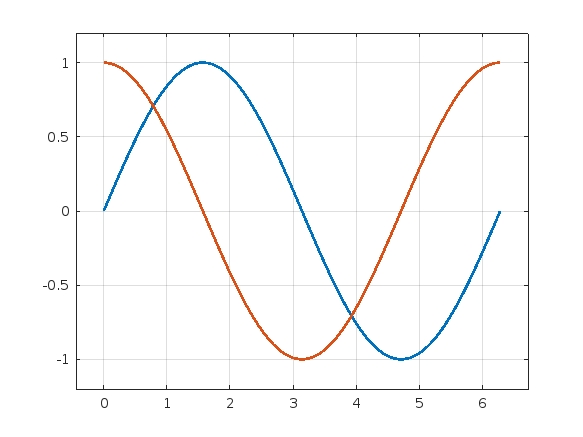
Here is a standard MATLAB plot:
x = 0:pi/100:2*pi;
y1 = sin(x);
y2 = cos(x);
plot(x,y1,x,y2)

I don't like some aspects of this plot, and so I have put the following code into my startup file.
set(groot,"DefaultLineLineWidth",2)
set(groot,"DefaultAxesXLimitMethod","padded")
set(groot,"DefaultAxesYLimitMethod","padded")
set(groot,"DefaultAxesZLimitMethod","padded")
set(groot,"DefaultAxesXGrid","on")
set(groot,"DefaultAxesYGrid","on")
set(groot,"DefaultAxesZGrid","on")
With those defaults changed, here is my preferred appearance:
plot(x,y1,x,y2)
To develop uifigure-based app, I wish MATLAB can provide something like uiquestdlg to replace questdlg without changing too much of the original code developed for figure-based app. Also, uiinputdlg <-> inputdlg and so on.
It is time to support the cameraIntrinsics function to accept a 3-by-3 intrinsic matrix K as an input parameter for constructing the object. Currently, the built-in cameraIntrinsics function can only be constructed by explicitly specifying focalLength, principalPoint, and imageSize. This approach has drawbacks, as it is not very intuitive. In most application scenarios, using the intrinsic matrix
K=[fx,0,cx;
0,fy,cy;
0,0,1]
is much more straightforward and effective!
intrinsics = cameraIntrinsics(K)
Learn the basic of quantum computing, how to simulate quantum circuits on MATLAB and how to run them on real quantum computers using Amazon Braket. There will also be a demonstration of machine learning using quantum computers!

Details at MATLAB-AMAZON Braket Hands-on Quantum Machine Learning Workshop - MATLAB & Simulink. This will be led by MathWorker Hossein Jooya.
I kicked off my own exploration of Quantum Computing in MATLAB a year or so ago and wrote it up on The MATLAB Blog: Quantum computing in MATLAB R2023b: On the desktop and in the cloud » The MATLAB Blog - MATLAB & Simulink. This made use of the MATLAB Support Package for Quantum Computing - File Exchange - MATLAB Central
Good day I am looking someone to help me on the matlab and simulink I am missing some explanations.For easy communication you can contact 0026876637042
Recently my iMac became sluggish. I checked Activity Monitor and found it was spending most of its time in mds_stores. I turned of Apple Intelligence under System Settings - Apple Intelligence & Siri, and its like new again.
Do you boast about the energy savings you racking up by using dark mode while stashing your energy bill savings away for an exotic vacation🌴🥥? Well, hold onto your sun hats and flipflops!
A recent study presented at the 1st Internaltional Workshop on Low Carbon Computing suggests that you may be burning more ⚡energy⚡ with your slick dark displays 💻[1].
In a 2x2 factorial design, ten participants viewed a webpage in dark and light modes in both dim and lit settings using an LCD monitor with 16 brightness levels.
- 80% of participants increased the monitor's brightness in dark mode [2]
- This occurred in both lit and dim rooms
- Dark mode did not reduce power draw but increasing monitor brightness did.
The color pixels in an LCD monitor still draw voltage when the screen is black, which is why the monitor looks gray when displaying a pure black background in a dark room. OLED monitors, on the other hand, are capable of turning off pixels that represent pure black and therefore have the potential to save energy with dark mode. A 2021 Purdue study estimates a 3%-9% energy savings with dark mode on OLED monitors using auto-brightness [3]. However, outside of gaming, OLED monitors have a very small market share and still account for less than 25% within the gaming world.
Any MATLAB users out there with OLED monitors? How are you going to spend your mad cash savings when you start using MATLAB's upcoming dark theme?
- BBC study: https://www.sicsa.ac.uk/wp-content/uploads/2024/11/LOCO2024_paper_12.pdf
- BBC blog article https://www.bbc.co.uk/rd/articles/2025-01-sustainability-web-energy-consumption
- 2021 Purdue https://dl.acm.org/doi/abs/10.1145/3458864.3467682
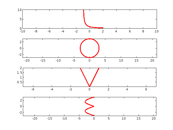
tiledlayout(4,1);
% Plot "L" (y = 1/(x+1), for x > -1)
x = linspace(-0.9, 2, 100); % Avoid x = -1 (undefined)
y =1 ./ (x+1) ;
nexttile;
plot(x, y, 'r', 'LineWidth', 2);
xlim([-10,10])
% Plot "O" (x^2 + y^2 = 9)
theta = linspace(0, 2*pi, 100);
x = 3 * cos(theta);
y = 3 * sin(theta);
nexttile;
plot(x, y, 'r', 'LineWidth', 2);
axis equal;
% Plot "V" (y = -2|x|)
x = linspace(-1, 1, 100);
y = 2 * abs(x);
nexttile;
plot(x, y, 'r', 'LineWidth', 2);
axis equal;
% Plot "E" (x = -3 |sin(y)|)
y = linspace(-pi, pi, 100);
x = -3 * abs(sin(y));
nexttile;
plot(x, y, 'r', 'LineWidth', 2);
axis equal;
On 27th February María Elena Gavilán Alfonso and I will be giving an online seminar that has been a while in the making. We'll be covering MATLAB with Jupyter, Visual Studio Code, Python, Git and GitHub, how to make your MATLAB projects available to the world (no installation required!) and much much more.
Sign up (it's free!) at MATLAB Without Borders: Connecting your Projects with Python and other Open-Source Tools - MATLAB & Simulink

Of course
62.5%
I never tried
37.5%
16 个投票
Check out the result of "emoji matrix" multiplication below.
- vector multiply vector:
a = ["😁","😁","😁"]
b = ["😂";
"😂"
"😂"]
c = a*b
d = b*a
- matrix multiply matrix:
matrix1 = [
"😀", "😃";
"😄", "😁"]
matrix2 = [
"😆", "😅";
"😂", "🤣"]
resutl = matrix1*matrix2
enjoy yourself!
I am looking for a Simulink tutor to help me with Reinforcement Learning Agent integration. If you work for MathWorks, I am willing to pay $30/hr. I am working on a passion project, ready to start ASAP. DM me if you're interested.
Bitte um Hilfe beim Kauf
I love it all
45%
Love the first snowfall only
15%
Hate it
17.5%
It doesn't snow where I live
22.5%
40 个投票
Since May 2023, MathWorks officially introduced the new Community API(MATLAB Central Interface for MATLAB), which supports both MATLAB and Node.js languages, allowing users to programmatically access data from MATLAB Answers, File Exchange, Blogs, Cody, Highlights, and Contests.
I’m curious about what interesting things people generally do with this API. Could you share some of your successful or interesting experiences? For example, retrieving popular Q&A topics within a certain time frame through the API and displaying them in a chart.
If you have any specific examples or ideas in mind, feel free to share!
For Valentine's day this year I tried to do something a little more than just the usual 'Here's some MATLAB code that draws a picture of a heart' and focus on how to share MATLAB code. TL;DR, here's my advice
- Put the code on GitHub. (Allows people to access and collaborate on your code)
- Set up 'Open in MATLAB Online' in your GitHub repo (Allows people to easily run it)
I used code by @Zhaoxu Liu / slandarer and others to demonstrate. I think that those two steps are the most impactful in that they get you from zero to one but If I were to offer some more advice for research code it would be
3. Connect the GitHub repo to File Exchange (Allows MATLAB users to easily find it in-product).
4. Get a Digitial Object Identifier (DOI) using something like Zenodo. (Allows people to more easily cite your code)
There is still a lot more you can do of course but if everyone did this for any MATLAB code relating to a research paper, we'd be in a better place I think.
Here's the article: On love and research software: Sharing code with your Valentine » The MATLAB Blog - MATLAB & Simulink
What do you think?
On my computers, this bit of code produces an error whose cause I have pinpointed,
load tstcase
ycp=lsqlin(I, y, Aineq, bineq);
Error using parseOptions
Too many output arguments.
Error in lsqlin (line 170)
[options, optimgetFlag] = parseOptions(options, 'lsqlin', defaultopt);
^^^^^^^^^^^^^^^^^^^^^^^^^^^^^^^^^^^^^^^^^^^
The reason for the error is seemingly because, in recent Matlab, lsqlin now depends on a utility function parseOptions, which is shadowed by one of my personal functions sharing the same name:
C:\Users\MWJ12\Documents\mwjtree\misc\parseOptions.m
C:\Program Files\MATLAB\R2024b\toolbox\shared\optimlib\parseOptions.m % Shadowed
The MathWorks-supplied version of parseOptions is undocumented, and so is seemingly not meant for use outside of MathWorks. Shouldn't it be standard MathWorks practice to put these utilities in a private\ folder where they cannot conflict with user-supplied functions of the same name?
It is going to be an enormous headache for me to now go and rename all calls to my version of parseOptions. It is a function I have been using for a long time and permeates my code.